Foreword
This document is a technical appendix to the MASTER report on the sea of Calabria. It reports in detail the biogeochemical analysis carried out in May 2026 to close what, until then, was a recognised gap in the mucilage analyses: the lack of a quantification of the third triggering factor (nutrients), in addition to the thermal factor (SST) and the mechanical one (wind + bathymetry) already analysed in the previous reports.
The analysis starts from a specific question: does the Calabrian Tyrrhenian coast, perceived by part of public opinion as a 'sewer' compared with the Ionian, present high nutrient values that would justify that perception? Or, on the contrary, does it have a chemical-biological profile that refutes the argument? The answer — which we will see in the following chapters — is scientifically clear-cut and overturns several commonplaces.
The structure of the document is as follows. Chapter 1 summarises the research question and the reason why it was necessary to add this third dimension. Chapter 2 explains how we selected the appropriate Copernicus Marine dataset, through a systematic probe of the available IDs. Chapter 3 — the most important for anyone wishing to judge the reliability of the work — describes in depth HOW Copernicus produces these data, what the uncertainties are, and which uses are legitimate. Chapter 4 documents the technical download and aggregation pipeline. Chapters 5, 6 and 7 present, respectively, the comparison between the four coasts, the 1999-2024 historical series for the Amantea-Lamezia stretch, and the 3-factor composite index. Chapter 8 discusses the practical implications, in particular for the public narrative on the Tyrrhenian. Chapter 9 lists the limitations of the analysis and future developments.
All the work is reproducible: the analysis script (mucillagini_bgc.py) is in the project, the Copernicus data are public (upon free registration), and the charts and tables reported here are generated automatically by the same script. The 5 local NetCDF caches (one per zone) weigh in total about 1 MB and make it possible to re-run the analyses without re-downloading the data.
Glossary of the abbreviations and indicators used
This technical appendix uses several chemical abbreviations, biological shorthand, specialist units of measurement and institutional acronyms. To make the reading accessible also to those without technical training in oceanography or water chemistry, the full explanations are provided below, with the meaning of each abbreviation, the associated unit of measurement, and — above all — the reason why that particular parameter is analysed.
Dissolved nutrients and chemical-biological indicators
| Abbreviation / Term | What it is and why it is analysed |
|---|---|
| NO₃ (nitrate, also written NO3) | The anion of the salt of nitric acid. It is the most oxidised form of nitrogen dissolved in the sea and is the main source of nitrogen usable by phytoplankton to build proteins. IT IS ANALYSED BECAUSE: high concentrations indicate human inputs (treated sewage discharges, agricultural fertilisers washed down by rivers); low concentrations indicate the oligotrophy typical of the Mediterranean. Unit: μM (micromoles per litre) or mmol/m³ (millimoles per cubic metre) — equivalent for dilute aqueous solutions. Typical 'clean sea' limit for the Mediterranean: <1 μM. |
| NH₄ (ammonium, also written NH4) | The most reduced form of dissolved nitrogen, produced by the decomposition of organic matter or present directly in untreated sewage discharges. IT IS ANALYSED BECAUSE: it is the real 'chemical tracer' of fresh faecal discharges, because it otherwise transforms rapidly into NO₃. In our study we did not use it as the main indicator because it is very noisy at the Mediterranean scale. |
| PO₄ (phosphate, also written PO4 or orthophosphate) | The anion of the salt of phosphoric acid. It is the main source of phosphorus usable by phytoplankton (the other essential element besides nitrogen). IT IS ANALYSED BECAUSE: the Mediterranean is structurally phosphorus-deficient, and this determines what 'controls' the growth of the algae. Domestic discharges (soaps, detergents) and agricultural fertilisers locally increase PO₄. Unit: μM or mmol/m³. Typical clean-sea value: <0.05 μM. Below 0.01 μM one is in conditions of strong limitation. |
| N:P ratio | The molar ratio between the nitrate concentration and the phosphate concentration, computed as N:P = [NO₃] / [PO₄]. An indicator of chemical IMBALANCE: phytoplankton needs N and P in a fixed ratio of ~16:1 (see Redfield), so if it finds a very different ratio it enters a state of stress. IT IS ANALYSED BECAUSE: N:P values >> 16 indicate 'phosphorus limitation' (typical of the Mediterranean) and therefore potential phytoplankton stress, a producer of EPS — the 'building blocks' of mucilage. |
| Redfield ratio (16:1) | The optimal molar ratio between nitrogen and phosphorus in marine biomass, discovered by the oceanographer Alfred Redfield in the 1930s. Phytoplankton 'in balance' takes up N and P in a 16:1 ratio. Values well above or below this ratio indicate environmental imbalances. |
| NPP / NPPV (Net Primary Productivity / Volume integrated) | How much carbon (in the form of new biomass) the phytoplankton fixes each day per cubic metre of water through photosynthesis, net of how much it consumes in respiration. It is the 'growth rate' of the phytoplankton in the photic layer. IT IS ANALYSED BECAUSE: it is a direct proxy of phytoplankton biomass and of EPS production. Unit: mgC/m³/day (milligrams of carbon fixed per cubic metre of water per day). Typical Mediterranean values: 5-15 mgC/m³/day. |
| EPS (Extracellular Polysaccharides) | Complex sugars released by phytoplankton under stress. IT IS ANALYSED BECAUSE: they are the biological 'building blocks' of mucilage — when they aggregate into TEP particles (see below) they produce macroscopic masses. |
| TEP (Transparent Exopolymer Particles) | Transparent gelatinous particles formed by the aggregation of EPS in marine waters. IT IS ANALYSED BECAUSE: they are the precursor aggregation state of visible mucilage. |
| CHL (Chlorophyll-a) | The green photosynthetic pigment characteristic of all algae and plants. Its concentration in water is proportional to the phytoplankton biomass. IT IS ANALYSED BECAUSE: it is the most reliable proxy of the quantity of algae in the sea. It is measured directly from satellites (ocean colour: chlorophyll alters the colour of the water in the blue-green). Unit: mg/m³ (milligrams per cubic metre). Typical values for an oligotrophic open sea: 0.05-0.15 mg/m³; for a eutrophic coast: over 1 mg/m³. |
| KD490 (Diffuse Attenuation Coefficient at 490 nm) | The light attenuation coefficient at the 490 nm wavelength (blue-green). It measures HOW RAPIDLY light is absorbed as it descends through the water. IT IS ANALYSED BECAUSE: it is the standard satellite proxy of the TURBIDITY of coastal waters. Clear water (low KD490, ~0.02 m⁻¹) = light penetrates; turbid water with particulates/algae/discharges (high KD490, >0.1 m⁻¹) = light absorbed rapidly. Unit: m⁻¹ (inverse of metres). |
| pH (potential of hydrogen) | A logarithmic measure of the acidity of a solution, from 0 (extremely acidic) to 14 (extremely basic). Sea water is naturally slightly alkaline (pH ≈ 8.0-8.2). IT IS ANALYSED BECAUSE: the absorption of anthropogenic CO₂ from the atmosphere progressively lowers the pH of the sea ('marine acidification'). A change of 0.1 pH units = double the concentration of hydrogen ions (logarithmic scale). |
| TALK / Total alkalinity | The capacity of water to neutralise acids (buffering capacity). It measures the concentration of carbonates, bicarbonates and other alkaline ions. IT IS ANALYSED BECAUSE: it indicates the 'strength' of the marine buffer system against acidification. Higher alkalinity = greater buffering capacity. Unit: mol/m³ (moles per cubic metre). |
| DIC / DISSIC (Dissolved Inorganic Carbon) | Total dissolved inorganic carbon: the sum of CO₂, bicarbonate ions (HCO₃⁻) and carbonate ions (CO₃²⁻). IT IS ANALYSED BECAUSE: it measures how much total carbon is dissolved in the sea; together with pH and alkalinity it completely defines the carbonate system. |
| Salinity (so, also written S) | The quantity of dissolved salts in the water. IT IS ANALYSED BECAUSE: it indicates inputs of fresh water (discharges, rivers, intense rainfall). Atlantic water is less salty, Mediterranean water saltier. Local variations may indicate land inputs. Unit: PSU (Practical Salinity Unit), a dimensionless scale calibrated on conductivity ratios. Typical Mediterranean: 37-39 PSU. |
Units of measurement used
| Unit | What it means |
|---|---|
| μM (micromolar) | Molar concentration: the number of micromoles of a substance per litre of solution. 1 μM = 1 micromole/litre = 10⁻⁶ moles/litre. For dilute aqueous solutions (such as sea water), 1 μM ≈ 1 mmol/m³. Used to express nutrient concentrations. |
| mmol/m³ (millimoles per cubic metre) | A unit equivalent to μM for aqueous solutions. It is the SI base unit for concentrations in the sea. |
| mol/m³ (moles per cubic metre) | A 'larger' unit: 1 mol/m³ = 1000 mmol/m³. Used for total alkalinity and DIC, which are higher concentrations (~2.6 mol/m³ typical). |
| mg/m³ (milligrams per cubic metre) | A mass concentration. 1 mg/m³ ≈ 1 μg/litre = 1 part per billion. Used for chlorophyll. |
| mgC/m³/day | The mass of carbon (in milligrams) fixed through photosynthesis per cubic metre of water per day. It is the primary-production flux. |
| m⁻¹ (per metre, inverse) | The attenuation coefficient: it describes how much light is absorbed per unit of depth. Higher = more turbid water. |
| PSU (Practical Salinity Units) | A dimensionless salinity scale based on electrical-conductivity ratios. Typical Mediterranean values: 37-39. |
| cfu/100ml (colony forming units) | A counting unit in microbiology. The number of bacterial colonies that form in 100 ml of water after plate culture. Used for the regulatory limits of E. coli (500 cfu/100ml) and enterococci (200 cfu/100ml). |
Technical acronyms, institutions and data products
| Acronym | Meaning and role |
|---|---|
| BGC (Biogeochemistry) | The study of chemical and biological cycles in marine ecosystems. The Copernicus 'BGC data' include nutrients, oxygen, chlorophyll, carbonates and phytoplankton biomass. |
| MedBFM (Mediterranean BioGeoChemical Flux Model) | A numerical model that simulates the biogeochemistry of the Mediterranean. Developed and maintained by OGS (Trieste) in collaboration with CMCC. It is the source of our data on nutrients, NPP, pH and alkalinity. |
| BFM (Biogeochemical Flux Model) | The biological-chemical core of the model: it simulates the interactions between phytoplankton (4 groups), zooplankton (3 groups), bacteria and the nutrient cycles. |
| NEMO (Nucleus for European Modeling of the Ocean) | The physical ocean-circulation model used as the basis for MedBFM. It simulates temperature, salinity and three-dimensional currents. |
| Med-MFS (Mediterranean Forecasting System) | The operational forecasting system of the Mediterranean based on NEMO. It provides our surface-salinity data. |
| Ocean Colour | A generic term for the satellite observations that measure the colour of the sea. From this measurement, chlorophyll and turbidity are derived. Sensors: MODIS-Aqua, Sentinel-3 OLCI, VIIRS, SeaWiFS. |
| L3 / L4 (Level 3 / Level 4) | Processing levels of satellite data. L3 = a regular grid with possible gaps (clouds). L4 = a gap-free interpolated grid (no holes), produced by combining several satellites and interpolation algorithms. |
| REP (Reprocessed) | A variant of the Copernicus data produced by applying consistent algorithms to the whole historical series. Used for long-term climate analyses. Publication lag: ~4-5 months. |
| NRT (Near Real Time) | A variant of the Copernicus data published with a lag of 24-48 hours. Used for operational monitoring, statistically less robust. |
| RMSE (Root Mean Square Error) | A statistical measure of the error of a model. It is the square root of the mean of the squared deviations between model and observations. Expressed as a percentage or in the same units as the variable. |
| CMEMS (Copernicus Marine Environment Monitoring Service) | The European Union's marine monitoring service (Copernicus programme). It freely distributes over 200 oceanographic datasets. |
| OGS (National Institute of Oceanography and Experimental Geophysics) | An Italian research body based in Trieste, the developer of the MedBFM model. Among the largest Italian oceanographic institutes. |
| CMCC (Euro-Mediterranean Center on Climate Change) | An Italian research foundation based in Lecce, an OGS partner for the development of the Med-MFS+BFM reanalysis. |
| ARPACAL (Regional Environmental Protection Agency of Calabria) | The Calabrian public body that officially carries out the sampling and analyses for bathing (Directive 2006/7/EC, Legislative Decree 116/2008). Accredia-accredited laboratories. |
| BGC-Argo | An international network of autonomous floats (~30 active in the Mediterranean) that measure in situ oxygen, chlorophyll, nitrates and pH down to 2000 m depth. Used to validate MedBFM. |
| EMODnet (European Marine Observation and Data Network) | A European aggregate of all historical marine in-situ observations, used to validate the biogeochemical models. |
| ISPRA | The Italian Higher Institute for Environmental Protection and Research. The Italian reference body for national environmental monitoring. |
In the chapters that follow, each time an abbreviation appears for the first time in the text, it is written accompanied by its full meaning. For later reference one can always return to this glossary.
1. The research question
1.1 The three triggering factors of mucilage
The scientific literature on Mediterranean mucilage is fairly well established. The phenomenon requires the temporal coincidence of FOUR conditions, three of which are measurable with remote-sensing or modelling data:
| Factor | What is needed | Source of measurement | Status |
|---|---|---|---|
| Thermal | SST > 22 °C early, stable thermal stratification | Satellite SST (Copernicus L4 REP) | Analysed in the previous reports (Ch. 3 of the MASTER) |
| Mechanical | A calm sea for >10-15 consecutive days, weak wind | Satellite wind + GWA for validation | Analysed in the previous reports (Ch. 4 of the MASTER) |
| Nutritive | An input of N and P in the pre-season months + summer phytoplankton stress | Copernicus MedBFM biogeochemical model | ANALYSED IN THIS DOCUMENT |
| Biological | A predisposed phytoplankton community, the absence of predators | Direct sampling and microscopy | Not available from satellite/model — out of scope |
The biological factor (the phytoplankton community) is not measurable with satellite or modelling data at the Mediterranean scale: it requires specific direct sampling, beyond the reach of this study. The other three, on the other hand, are all accessible. Until now only the third (nutritive) was missing to complete the picture.
1.2 The specific question for the Tyrrhenian
In popular posts and public discussions about the Calabrian sea, one argument recurs frequently: 'the Tyrrhenian is a sewer'. It is an argument based mainly on the visual observation of the summer mucilage phenomena, which it attributes to pollution from discharges.
The precise scientific question we ask is: are the dissolved nutrients in the surface layer of the Calabrian Tyrrhenian sea actually HIGH (compatible with a hypothesis of significant human pressure via untreated discharges) or LOW (incompatible with that hypothesis and compatible instead with normal Mediterranean oligotrophy)? The answer has direct implications for policy and for public communication.
If the Tyrrhenian nutrients turned out to be higher than the Ionian ones, the 'hunt for the illegal pipe' argument would have a foundation. If they turned out to be equal or, paradoxically, lower, the argument would prove unfounded. We will see in Chapter 5 that the reality is the second — and clearly so.
2. Probe and selection of the Copernicus BGC dataset
2.1 The Copernicus Marine BGC catalogue for the Mediterranean
The Copernicus Marine Environment Monitoring Service (CMEMS) publishes several biogeochemical datasets for the Mediterranean. Before proceeding with the download, a systematic probe was necessary to identify which datasets were actually available and which variables they contained, because the nomenclature changes between versions and some datasets documented in the literature are no longer active in the current catalogue.
6 candidates were tested through a small remote-opening script (without downloading the full volume, only the metadata). The probe results:
| Dataset ID | Main variables | Probe result |
|---|---|---|
| cmems_mod_med_bgc-pft_my_4.2km_P1D-m | Plankton Functional Types (chlorophyll by group) | DatasetNotFound |
| cmems_mod_med_bgc-nut_my_4.2km_P1D-m | Nutrients (NH4, NO3, PO4) | OK — variables confirmed, 125 vertical levels |
| cmems_mod_med_bgc-pft_myint_4.2km_P1M-m | Monthly PFT climatology | DatasetNotFound |
| cmems_mod_med_bgc-nut_myint_4.2km_P1M-m | Monthly nutrient climatology | DatasetNotFound |
| cmems_mod_med_bgc-bio_my_4.2km_P1D-m | Biology (NPP, oxygen) | OK — nppv + o2 available |
| cmems_mod_med_bgc-car_my_4.2km_P1D-m | Carbonates (DIC, pH, alkalinity) | OK — but not relevant for mucilage |
2.2 The choice of the two operational datasets
Of the 6 candidates, 3 turned out to be available and 3 no longer exist in the current catalogue (a 'DatasetNotFound' error). Among the 3 available, we chose the two most relevant for mucilage:
- cmems_mod_med_bgc-nut_my_4.2km_P1D-m for the nutrients — it provides the concentrations of nitrate (NO3), phosphate (PO4) and ammonium (NH4) in the water column. For our analysis NO3 and PO4 are needed: their N:P ratio is the indicator of phytoplankton stress from nutrient limitation.
- cmems_mod_med_bgc-bio_my_4.2km_P1D-m for the biology — it provides the net volume-integrated primary productivity (NPPV, in mg of carbon fixed per cubic metre per day) and the dissolved oxygen. For our analysis NPPV is needed as a direct proxy of the phytoplankton biomass in the photic layer.
The carbonate dataset (DIC, pH, alkalinity) was left out: these parameters concern marine acidification, a real and important phenomenon but not directly linked to the mechanism of mucilage.
2.3 Technical characteristics of the chosen datasets
| Characteristic | Value |
|---|---|
| Spatial resolution | 4.2 km × 4.2 km (0.04° on both axes) |
| Vertical resolution | 125 levels from 1 m to 4153 m |
| Temporal resolution | 1 daily mean value |
| Geographical coverage | The whole Mediterranean (lon -6° to 36.5°E, lat 30° to 46°N) |
| Temporal coverage | 1 January 1999 — 31 December 2024 (26 complete years) |
| Product version | Multiyear reanalysis, latest release: 202511 |
| NUT variables | no3, nh4, po4 (mmol/m³ = μM for dilute aqueous solutions) |
| BIO variables | nppv (mgC/m³/day), o2 (mmol/m³) |
| Availability | Free upon registration at marine.copernicus.eu |
The daily granularity is important: it allows us to capture short-lived summer peaks that a monthly climatology would mask. The 125-level vertical resolution allows us to extract precisely the photic surface layer (0-10 m) — where mucilage actually occurs, not at 4000 m depth.
3. Reliability of the data: how the MedBFM model works
This is the most important chapter for judging the robustness of the study. Unlike satellite SST — which is a direct measurement — the biogeochemical data have a complex production pathway and require care in their use.
3.1 The fundamental difference relative to SST
When a satellite measures SST, it does so through sensors that directly read the thermal radiation emitted by the sea surface. The measurement is physical, direct, and the stated accuracy (~0.2-0.3 °C) is verified against thousands of reference oceanographic buoys every year. When we see in the MASTER report that the summer SST of 2024 was 27.3 °C, that number is a measurement, not an estimate.
The biogeochemical data are NOT direct measurements. One cannot 'see' a nitrate at 2 metres depth with a satellite sensor: nitrates do not emit characteristic radiation. To obtain the concentration values, a NUMERICAL MODEL is used that simulates the biogeochemical reactions of the sea on a computer, with all the pros and cons that this entails.
3.2 The Med-BFM model (OGS Trieste)
The biogeochemical model used by Copernicus for the Mediterranean is called Med-BFM — Mediterranean BioGeoChemical Flux Model. It is developed and maintained by OGS — the National Institute of Oceanography and Experimental Geophysics of Trieste, one of the main Italian research centres in oceanography, in collaboration with the Euro-Mediterranean Center on Climate Change Foundation (CMCC).
Med-BFM works coupled to two main components:
- A physical oceanographic model (NEMO-MFS) that simulates the circulation of the Mediterranean water masses — temperature, salinity, three-dimensional currents, vertical mixing. NEMO is the same model used for the Copernicus meteo-marine forecasts, and it is a world standard.
- A biogeochemical model (BFM, Biogeochemical Flux Model) that, on top of the physical framework, simulates the chemical-biological reactions: 4 groups of phytoplankton (diatoms, flagellates, picophytoplankton, dinoflagellates), 3 of zooplankton (microzooplankton, mesozooplankton, predators), heterotrophic bacteria, dissolved and particulate organic matter, oxygen, the carbon cycle, the nutrient cycles (N, P, Si). In total, about 50 state variables are simulated simultaneously for each pixel.
For each pixel of the Mediterranean grid (~70,000 points × 125 vertical layers = ~9 million 3D cells), the model numerically solves the differential equations that describe how nutrients, photosynthesis, respiration and the sedimentation of organic material evolve over time. It computes hour by hour, for 26 years of simulation. It is a computationally very heavy calculation: it runs on a supercomputer at CINECA (Bologna) and takes weeks to produce a complete reprocessing of the historical series.
3.3 Data assimilation: how the errors are corrected
A numerical model, left to itself for 26 years of simulation, tends to drift away from reality ('model drift'). The small initial imprecisions accumulate, the simplified equations introduce systematic errors, and complex biological parameters (such as photosynthesis under stress) are modelled with approximations. For this reason Copernicus applies so-called data assimilation: the model is periodically 'corrected' with the real observational data available.
The four main observational sources used for the calibration of Med-BFM are:
- Satellite chlorophyll (ocean colour). Sensors such as MODIS-Aqua, Sentinel-3 OLCI and VIIRS measure the colour of the sea seen from above. The quantity of chlorophyll in the first metres of water alters this colour in a predictable way, and from there the chlorophyll concentration is computed with well-characterised accuracy. This measurement is used to 'put back on track' the phytoplankton simulated by the model, typically every 7-10 days.
- BGC-Argo floats. These are autonomous floats (~30 active in the Mediterranean in 2024) that descend down to 2000 m depth and measure in situ oxygen, chlorophyll, nitrates and pH, roughly every 10 days. They provide real vertical profiles against which the model can be validated.
- Oceanographic campaigns on Italian ships (CNR, OGS, INGV), French (Ifremer), and Spanish (CSIC). Ships such as the Urania, Minerva Uno and Dallaporta periodically carry out standardised transects with seasonal water samples at various depths, analysed in the laboratory for precise concentrations.
- The European EMODnet aggregate (European Marine Observation and Data Network), which collects and harmonises all the historical chemical/biological in-situ measurements of the Mediterranean from the 1960s onwards.
The final product we use in the mucillagini_bgc.py script is therefore a model that is NUMERICAL BUT CALIBRATED on observed reality: neither a blind simulation nor a direct measurement. It is a middle ground, which has its own specific uncertainties.
3.4 Validation and stated uncertainties
For each release of Med-BFM, Copernicus publishes an official document called the Product Quality Information Document (PQID) that reports the error metrics of the model compared with independent observational data. The typical uncertainties for the Mediterranean:
| Variable | Typical RMSE | Validation notes |
|---|---|---|
| Surface chlorophyll | ~30% | Validated against satellite ocean colour and BGC-Argo |
| Nitrates (NO3) | ~40% | Validated against EMODnet and ship campaigns |
| Phosphates (PO4) | ~35% | Validated against EMODnet and ship campaigns |
| Dissolved oxygen | ~10% | Validated against BGC-Argo (the most reliable variable) |
| Integrated NPP | ~30% | Validated indirectly via satellite chlorophyll |
| pH | ~5% | Validated against BGC-Argo, high reliability |
These uncertainties are significantly higher than those of SST (0.2-0.3 °C ≈ 1-2% on typical values). This is normal: we are trying to model complex and non-linear biological processes, against which the available observations are in any case sparse.
3.5 What can and what CANNOT be said from the BGC data
This is the most important section of the chapter. Rigorously defining what it is legitimate to assert on the basis of data with ~30-40% uncertainty is fundamental in order not to over-interpret the results. The golden rules:
| Type of statement | Reliability | Notes |
|---|---|---|
| Long-term trend (decades) | RELIABLE | The ~30% error is random; averaged over 26 years it cancels out. The up/down trends of NPP or nutrients are robust. |
| Mean spatial patterns (zone A vs zone B) | RELIABLE | The error is uniform across the domain. If zone A has NPP double that of zone B, the ratio remains true even with ±30% uncertainties in absolute value. |
| Seasonal patterns (January vs July) | RELIABLE | The model is calibrated precisely on seasonality via the assimilation of satellite chlorophyll, which captures the annual cycle well. |
| Specific year vs specific year | WITH CAUTION | The random uncertainty between years can exceed the signal. '2018 was worse than 2017' may be 60% true, not 95%. |
| A single point event | INSUFFICIENT | The 4.2 km resolution and the ~30% uncertainty are too large to predict local events in a specific bay. |
| A precise absolute value (e.g. NPP=7.15 mgC/m³/d) | TO BE AVOIDED | The number has an uncertainty of ~2 mgC/m³/d. We use it as a comparative indicator, not as a precise measurement. |
The Copernicus BGC data should not be used as an absolute measurement, but as a further comparative indicator to place alongside SST and wind. This is exactly what we did: add a third dimension to the ranking of the four coasts and of the historical years, not replace the other two. All the results presented in the following chapters are expressed in terms of percentile rank, anomaly or relative comparison — never as the 'absolute truth' of the single number.
4. Technical processing pipeline
4.1 The geographical box of the four zones
The four Calabrian coastal zones were defined with rectangular bounding boxes (latitude + longitude), consistent with those already used in the SST and wind analyses of the previous reports, so that the comparison is direct:
| Zone | Latitude (°N) | Longitude (°E) | Extremes and size |
|---|---|---|---|
| Tyrrhenian | 38.25 — 39.95 | 15.60 — 16.30 | Praia a Mare → Scilla, ~189 × 60 km |
| Far South | 37.85 — 38.25 | 15.55 — 16.30 | Scilla → Reggio Calabria → Bovalino, ~44 × 65 km |
| South Ionian | 37.95 — 39.05 | 16.30 — 17.20 | Capo Spartivento → Crotone, ~122 × 78 km |
| North Ionian | 39.05 — 39.95 | 16.55 — 17.20 | Crotone → Roseto Capo Spulico, ~100 × 50 km |
| Amantea-Lamezia | 38.88 — 39.18 | 15.90 — 16.28 | Focus on the southern Tyrrhenian stretch, ~33 × 33 km |
4.2 The download and cache script
The mucillagini_bgc.py script implements a linear pipeline in three phases: download, aggregation, indicator computation. For each zone the cm.open_dataset() method of copernicusmarine is called with the appropriate parameters. An example of the call for the nutrient dataset:
ds_nut = cm.open_dataset( dataset_id="cmems_mod_med_bgc-nut_my_4.2km_P1D-m", variables=["no3", "po4"], minimum_longitude=box["lon"][0], maximum_longitude=box["lon"][1], minimum_latitude=box["lat"][0], maximum_latitude=box["lat"][1], minimum_depth=0, maximum_depth=10.0, start_datetime="1999-01-01", end_datetime="2024-12-31", )
Immediately after the download, two aggregations drastically reduce the volume:
- Vertical aggregation: the mean of the values over the 0-10 m levels (the model returns ~6-7 levels in this band). A single value per horizontal pixel is obtained.
- Spatial aggregation: the areal mean of all the pixels of the box. A 1D time series of a single value per day for each variable is obtained.
The final result for each zone is a NetCDF of about 200 KB with three time series (NO3, PO4, NPP) of 9,497 daily values each (1999-01-01 → 2024-12-31). The 5 caches together occupy about 1 MB on disk. Re-runs of the script skip the download and use the cache.
4.3 Execution time
The complete download via the Copernicus Marine API took about 25 minutes for the 5 zones × 2 datasets = 10 calls. Most of the time is on the Copernicus server side, which assembles the requested subset; the network transfer is fast because the data are already aggregated to the 0-10m layer at the server. The pipeline is I/O bound, not CPU bound.
Subsequent reprocessing (changing formulas, new charts, different indices) starts from the local cache and takes <30 seconds in total for all the zones. This is the main reason why the local cache is fundamental for any serious analysis pipeline on Copernicus data.
5. Results: comparison between the four coasts
5.1 The 1999-2024 means by zone
Averaging the 26 years of biogeochemical data for each of the four Calabrian coasts, we obtain the following summary picture. The values represent the mean concentrations in the 0-10 m surface layer, computed over the indicated months.
| Biogeochemical indicator | Tyrrhenian | Far South | South Ionian | North Ionian |
|---|---|---|---|---|
| NO3 May-Jun (μM) | 0.503 | 0.555 | 0.588 | 0.596 |
| PO4 May-Jun (μM) | 0.009 | 0.009 | 0.006 | 0.005 |
| N:P ratio (Redfield = 16) | 59 | 73 | 102 | 119 |
| Summer NPP July-August (mgC/m³/d) | 7.15 | 7.70 | 8.52 | 10.36 |
| Summer-peak NPP May-Sep (mgC/m³/d) | 8.26 | 10.44 | 11.06 | 13.92 |
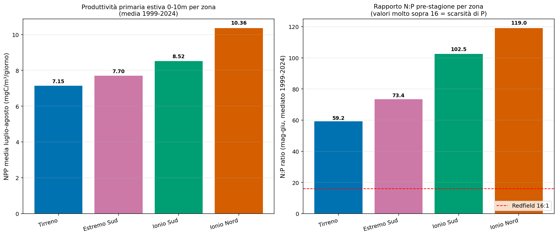
Figure 5.1 — Comparison of the four Calabrian coasts for summer primary productivity (left) and pre-season N:P ratio (right), 1999-2024 means from the MedBFM model. The Tyrrhenian → North Ionian gradient is clearly visible: nutrients and productivity increase as one moves from the Tyrrhenian towards the northern Ionian.
5.2 Reading the results: the Tyrrhenian-Ionian gradient
The data return a very clear and somewhat counter-intuitive picture. There is an evident west-east GRADIENT: moving from the Tyrrhenian towards the North Ionian, nutrients increase, the N:P ratio increases drastically (from 59 to 119, almost doubling), and the primary productivity increases (from 7.15 to 10.36 mgC/m³/day, +45%).
Three specific considerations:
- The Calabrian Tyrrhenian coast is the most OLIGOTROPHIC (nutrient-impoverished) of the four zones. Not only is it not a sewer: it has the lowest nutrient concentrations of the region; in particular the PO4 (0.009 μM), while well above the Redfield ratio of 16:1, has an absolute value that is in any case modest.
- The North Ionian has the highest N:P RATIO (119) — almost 8 times above the Redfield value. This means a severe shortage of phosphorus relative to nitrogen, which puts the phytoplankton under marked stress. It is typical of the eastern Mediterranean and of the Ionian basin, where the nitrogen inputs via the atmosphere and from the large rivers (Crati, Neto) are not balanced by adequate phosphorus inputs.
- The North Ionian also has the highest summer NPP (10.36 mgC/m³/d, +45% relative to the Tyrrhenian). Phytoplankton under stress produces a lot, but a large fraction of that biomass is composed of extracellular polysaccharides — the 'building blocks' of mucilage.
5.3 The apparent paradox and its explanation
If the Tyrrhenian has the lowest nutrients and the lowest NPP, why is it precisely the zone with the highest frequency of documented mucilage events? And if the North Ionian has the highest N:P ratio and NPP, why does it have very few events?
The answer is in the role of the mechanical factor (wind + bathymetry + currents), already discussed in detail in chapters 4.1-4.4 of the MASTER report. For visible mucilage it is not enough for the phytoplankton to produce polysaccharides: these must also ACCUMULATE at the surface. The accumulation requires a calm and stratified sea, because in a windy and dynamic sea the gelatinous particles disperse before aggregating into macroscopic masses.
The Tyrrhenian produces little 'raw material' but conserves it: a mean summer wind of 2.26 m/s (the lowest of the 4 coasts), a bathymetry with semi-enclosed gulfs (Sant'Eufemia above all), a wide continental shelf, a circulation with semi-stationary eddies. Everything conspires so that the EPS produced stay where they are. The North Ionian produces a lot of raw material but disperses it: wind of 2.74 m/s, a bathymetry with a more rapid drop, the passage of the Atlantic Ionian Stream that renews the surface waters. The EPS produced do not have time to aggregate.
The biogeochemical data demonstrate rigorously that the Tyrrhenian-Ionian difference in mucilage is NOT due to greater human pressure on the Tyrrhenian (because the Tyrrhenian nutrients are the lowest). It is due exclusively to the different physical-mechanical regime of the sea: wind, bathymetry, currents. The mechanical factor is dominant over the nutritive factor.
6. Historical series 1999-2024: the Amantea-Lamezia focus
6.1 Annual indicators
For the Amantea-Lamezia stretch — the historical focus of our mucilage analyses — the 1999-2024 series of annual indicators is as follows. We show the last 10 years for readability; the complete series is available in the file indicatori_bgc_amantea_lamezia.csv.
| Year | NO3 May-Jun | PO4 May-Jun | N:P ratio | NPP Jul-Aug | NPP summer max |
|---|---|---|---|---|---|
| 2015 | 0.508 | 0.008 | 66.0 | 7.22 | 8.38 |
| 2016 | 0.497 | 0.008 | 66.2 | 6.23 | 7.88 |
| 2017 | 0.556 | 0.009 | 64.8 | 6.10 | 7.80 |
| 2018 | 0.519 | 0.009 | 56.8 | 6.78 | 9.51 |
| 2019 | 0.507 | 0.009 | 55.1 | 6.06 | 7.64 |
| 2020 | 0.562 | 0.009 | 63.9 | 6.41 | 7.86 |
| 2021 | 0.536 | 0.008 | 63.9 | 6.77 | 8.33 |
| 2022 | 0.585 | 0.009 | 62.7 | 6.15 | 7.24 |
| 2023 | 0.463 | 0.007 | 70.5 | 6.99 | 8.99 |
| 2024 | 0.411 | 0.006 | 65.0 | 7.11 | 8.30 |
6.2 Trend and variability
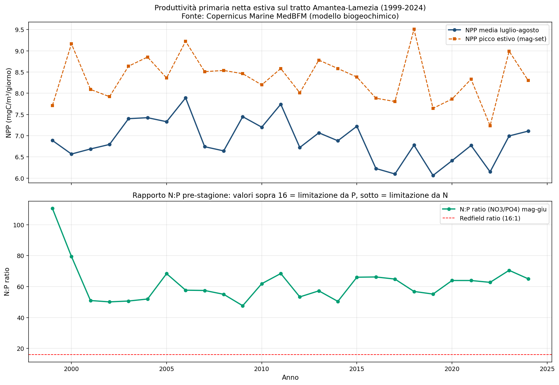
Figure 6.1 — Annual trend 1999-2024 on the Amantea-Lamezia stretch. Upper panel: net primary productivity (NPP), July-August mean and May-Sep summer peak. Lower panel: pre-seasonal N:P ratio, compared with the Redfield value of 16:1.
Three observations from reading the charts:
- The N:P ratio is ALWAYS well above the Redfield value: it oscillates between 50 and 110 throughout the period, with an anomalous peak in 1999 (110.5) and stable values around 60-70 in the last 10 years. It is consistent with the oligotrophic nature of the western Mediterranean, which is structurally phosphorus-deficient.
- The summer NPP is SLIGHTLY rising: from the 6.5 mgC/m³/d mean of the 2001-2010 period to the 6.8 mean of the 2015-2024 period. A modest increase (+5%) but statistically consistent with the marine warming: a warmer sea → more stable stratification → greater phytoplankton stress → more EPS produced.
- Isolated peak years: 1999 (N:P 110.5), 2005 (high summer NPP), 2011 (very high NPP), 2018 (NPP max 9.5), 2023 (recent record N:P 70.5). These are years in which the nutritive factor was particularly unfavourable.
6.3 Interannual variability vs long-term trend
The interannual variability is important: the N:P ratio goes from 55 (2019) to 70 (2023) — a 27% variation in 4 years. This variability is partly modelling-related (an uncertainty of ~35-40% on the absolute values), partly real (the anomalies of wind, rain and circulation change from year to year). Extracting a statistically significant trend requires averages over long periods.
For our analysis, however, the interannual variability is PRECISELY the interesting signal: it allows us to identify particular years (see Ch. 7) in which the meteo-marine and nutritive precursors aligned, creating potentially very favourable conditions for mucilage.
7. The 3-factor composite index
7.1 Construction of the index
Combining the historical series of SST, wind (already computed in the previous reports) and biogeochemistry (this analysis), we built a new 3-factor composite index for the Amantea-Lamezia stretch, expressed on a 0-100 scale where 100 represents the worst combination of mucilage precursors.
The two normalised components and their weights:
- THERMAL component (weight 50%): 40% mean May SST + 30% earliness of the first day with SST≥22 °C (in the year) + 30% number of days in the critical 24-28 °C window. Each sub-indicator is transformed into a percentile rank (0-100) over the whole series.
- NUTRITIVE component (weight 50%): 50% mean July-August NPP + 50% pre-season N:P ratio May-Jun. Here too, a percentile rank over the whole series.
The composite index is the weighted mean of the two components. Since the mechanical factor (wind) already influences the duration of the useful thermal window (and therefore enters into the thermal component), we decided not to add it as a separate third component to avoid double counting.
7.2 Results: Top 10 years by precursor preconditions
| Pos. | Year | Thermal comp. | Nutritive comp. | 3F index (new) | 2F index (old) |
|---|---|---|---|---|---|
| 1 | 2006 | 85.8 | 75.0 | 80.4 | 82.8 |
| 2 | 1999 | 67.1 | 78.8 | 73.0 | 74.8 |
| 3 | 2005 | 58.5 | 82.7 | 70.6 | 65.5 |
| 4 | 2011 | 47.1 | 92.3 | 69.7 | 55.8 |
| 5 | 2000 | 79.4 | 59.6 | 69.5 | 73.5 |
| 6 | 2024 | 58.8 | 71.2 | 65.0 | 60.8 |
| 7 | 2023 | 46.7 | 76.9 | 61.8 | 62.8 |
| 8 | 2007 | 79.6 | 42.3 | 61.0 | 80.9 |
| 9 | 2003 | 70.0 | 50.0 | 60.0 | 73.2 |
| 10 | 2015 | 35.8 | 76.9 | 56.3 | 42.0 |
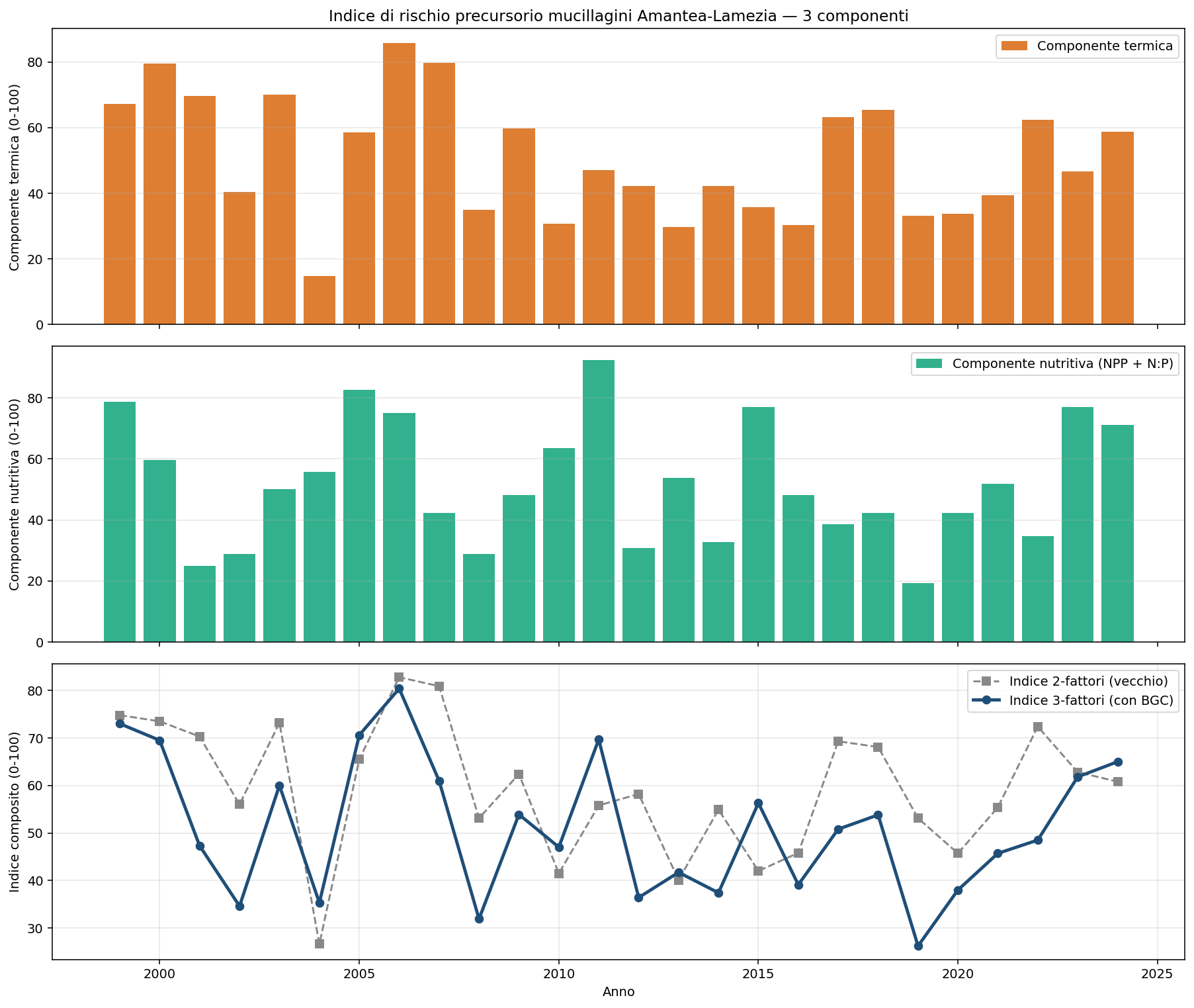
Figure 7.1 — Mucilage-precursor precondition index for Amantea-Lamezia in three panels. Panel 1: thermal component (0-100, percentile rank). Panel 2: nutritive component (0-100). Panel 3: comparison of the 2-factor index (grey, old) vs the 3-factor (blue, new).
7.3 What changes relative to the old 2-factor index
Adding the nutritive component does not overturn the ranking — 2006 remains firmly in first place (index 80.4 with 3 factors, 82.8 with the old 2 factors) — but it reshuffles the positions from 3rd to 10th, with four notable cases:
- 2011 rises from ~11th place to 4th place. The old index put it at 55.8 because the SST that year was modest. The new index brings it to 69.7 because the nutritive component is exceptional (92.3 out of 100 — the record of the series). This means that the biogeochemical model detected a high N:P imbalance together with one of the highest primary productivities. It is worth checking whether mucilage was documented locally that year.
- 2005 rises from 7th to 3rd place. A year with typical SST but high nutritive stress. Here too an interesting check with local operators.
- 2015 rises from ~18th to 10th place. A year with low SST but high nutritive stress (high N:P + high summer NPP).
- 2007 drops from 3rd to 8th place. It was a year with very high SST, but the BGC shows a moderate nutritive picture. Mucilage potentially less likely than estimated by the thermal indicator alone.
- 2003 also drops: it was 8th for SST alone, now it is 9th.
Adding the nutritive component, in summary, FILTERS the thermally warm but chemically moderate years (it demotes them) and PROMOTES the thermally average but chemically exceptional years. It captures a dimension that SST alone could not see.
7.4 Caveat on the interpretation
It must be said honestly that the 3-factor index is not a prediction of mucilage events. It is an indicator of PRECURSORS: it says how favourable the meteo-marine and chemical-biological conditions were to the formation of mucilage. To know whether in year X mucilage actually occurred, direct observations are needed (ARPA documents, photos, operator reports) that our study does not integrate. Also because the biological factor (the presence of the right species, the absence of predators) is not measurable via satellite or model.
That said, the added value of the index is methodological: it identifies WINDOWS OF FAVOURABLE CONDITIONS that deserve attention. In the years in the top 10 the probability of mucilage events is considerably higher than in the years at the bottom of the ranking.
8. Independent check with observational satellite chlorophyll
The biogeochemical data presented up to Chapter 7 all come from the MedBFM model. Those who read Chapter 3 carefully will remember that their official Copernicus uncertainty is ~30-40%. Good scientific practice requires that, when possible, the results of a model be compared with an INDEPENDENT OBSERVATION — possibly obtained with a completely different technology.
Chlorophyll, fortunately, is one of the few marine biogeochemical variables that can be measured directly from space. The photosynthetic pigment absorbs light in a characteristic way in the blue wavelengths (~440 nm) and reflects it in the green (~550 nm). Ocean-colour satellites (MODIS-Aqua, Sentinel-3 OLCI, VIIRS) measure this reflection spectrum and infer the surface chlorophyll concentration with well-characterised accuracy.
We therefore downloaded the Copernicus Ocean Colour Level-4 gap-free multi-sensor product at 1 km resolution, which integrates the observations of all the ocean-colour satellites available from 1997 to today and produces a daily gap-free map. It is an OBSERVATIONAL datum, not simulated — the ideal complement for verifying the results of the MedBFM model.
8.1 Dataset used
| Characteristic | Value |
|---|---|
| Dataset ID | cmems_obs-oc_med_bgc-plankton_my_l4-gapfree-multi-1km_P1D |
| Type | OBSERVATIONAL (NOT modelled) |
| Source sensors | MODIS-Aqua, Sentinel-3 OLCI, VIIRS, historical SeaWiFS |
| Variable | CHL = surface chlorophyll-a, mg/m³ |
| Spatial resolution | 1 km (4 times finer than the model) |
| Temporal resolution | 1 map per day (gap-free, no cloud holes) |
| Period covered | 1997 - today |
| Stated accuracy | RMSE ~30% (validated against in situ measurements) |
8.2 Results: comparison of the 4 zones (1999-2024 means)
| Observational CHL indicator | Tyrrhenian | Far South | South Ionian | North Ionian |
|---|---|---|---|---|
| Annual CHL (mg/m³) | 0.0899 | 0.1179 | 0.1142 | 0.1695 |
| Summer CHL Jun-Aug (mg/m³) | 0.0462 | 0.0598 | 0.0615 | 0.0870 |
| Winter CHL Jan-Mar (mg/m³) | 0.1563 | 0.1857 | 0.1772 | 0.2511 |
| CHL annual max (mg/m³) | 0.3205 | 0.6981 | 0.5319 | 0.7772 |
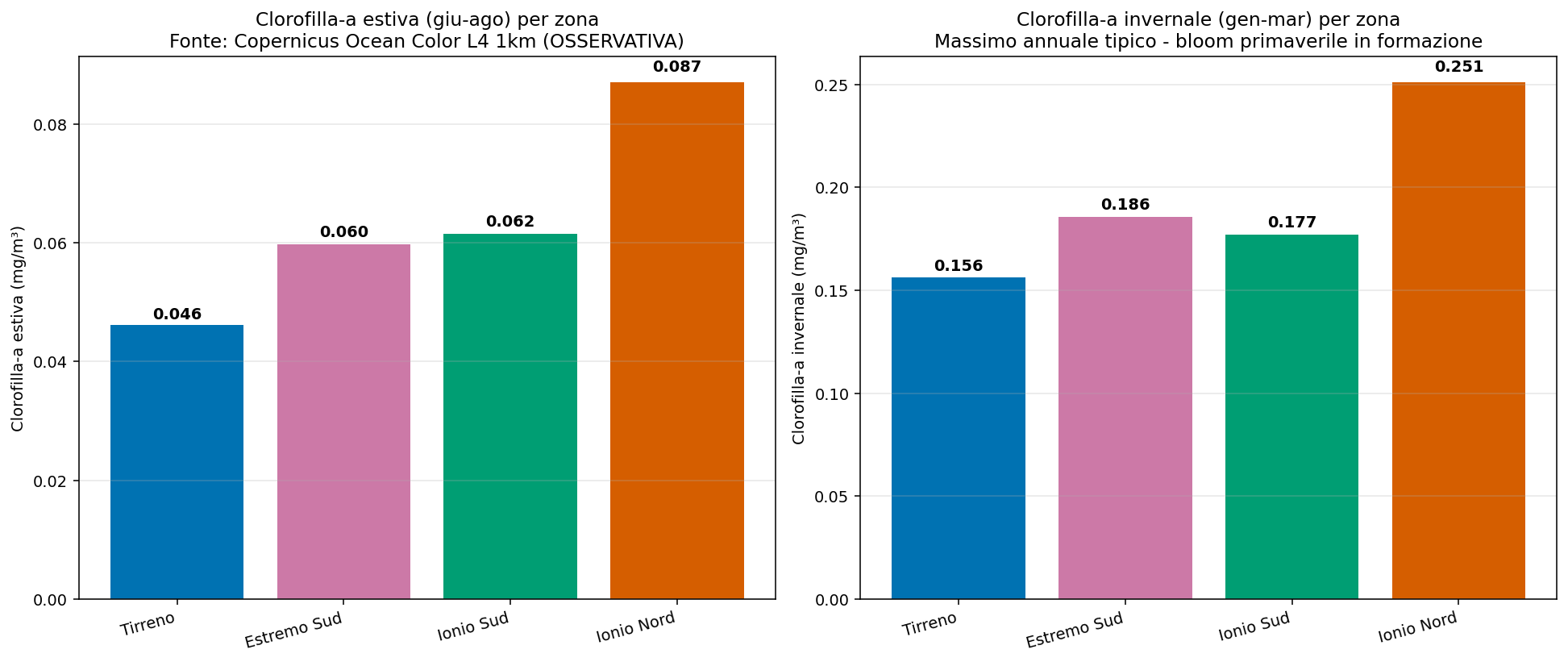
Figure 8.1 — Observational satellite chlorophyll-a by zone (summer and winter, 1999-2024 mean). Source: Copernicus Ocean Colour L4 1km, multi-sensor.
8.3 Reading: a total confirmation of the MedBFM model
The observational datum clearly CONFIRMS the pattern that emerged from the model: the North Ionian has the highest chlorophyll (annual 0.17 mg/m³, almost DOUBLE the Tyrrhenian), followed by the Far South and the South Ionian, with the Tyrrhenian at the MINIMUM (0.09 mg/m³). The exact same order that emerged from the MedBFM model for NPP (Ch. 5).
This is the best possible validation of the biogeochemical results: two completely different methodologies — a calibrated numerical model (MedBFM) and a direct optical satellite measurement (Ocean Colour) — agree on the same qualitative pattern and on a similar order of magnitude. It is not a fortunate coincidence, it is the real signal.
Direct implications for the Tyrrhenian:
- The summer observational chlorophyll of the Tyrrhenian is 0.046 mg/m³ — the LOWEST value of the four Calabrian coasts. It is the level typical of clean oligotrophic waters, not that of a sewer.
- The annual maximum peak too (CHL max, typically reached in the spring blooms) is the lowest: 0.32 mg/m³ against the 0.78 of the North Ionian. If there were significant discharges, there would be local and recurring chlorophyll peaks — they are not seen.
- The winter/summer ratio of the Tyrrhenian is about 3.4 — consistent with the natural annual cycle of Mediterranean phytoplankton (winter bloom, summer oligotrophy). If there were significant summer discharges from the large tourist flows, we would see an inversion or a flattening of the cycle. We do not see it.
Amantea-Lamezia trend 1999-2024
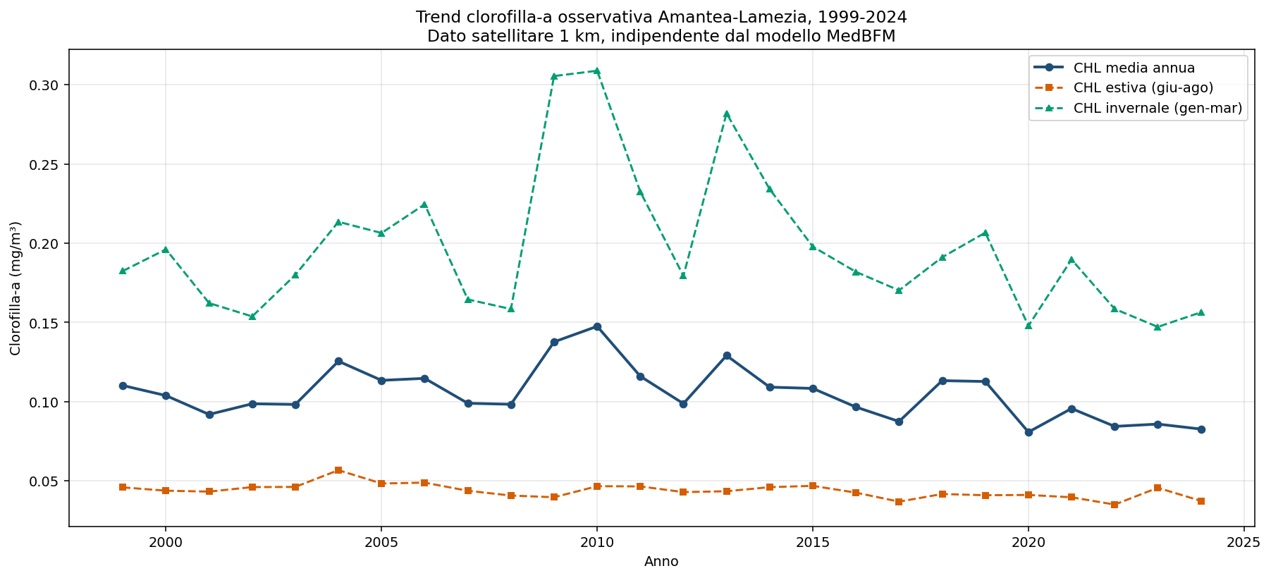
Figure 8.2 — Historical series of satellite chlorophyll on Amantea-Lamezia 1999-2024, broken down into annual, summer and winter means.
The historical series of Amantea-Lamezia shows considerable interannual variability but no clear growth trend: the summer CHL oscillates between 0.03 and 0.06 mg/m³ in the last 10 years, with no monotonic pattern. If there were a progressive deterioration from increasing human pollution, we would see a rising trend. There is none.
9. Marine acidification and buffering capacity (pH, alkalinity)
The second deeper analysis planned as a future development is the analysis of the carbonates: pH (the acidity of the water) and total alkalinity (the buffering capacity). These are global indicators of the marine acidification induced by the absorption of anthropogenic atmospheric CO2 — a phenomenon different from warming but linked to the same causes.
For the investigation of the Tyrrhenian, these indicators have a specific function: localised discharges of acidifying substances (malfunctioning treatment plants, industrial discharges, acidic discharges) would leave a signature of locally lower pH. A clean test for identifying any differential chemical pollution.
9.1 Dataset used
| Characteristic | Value |
|---|---|
| Dataset ID | cmems_mod_med_bgc-car_my_4.2km_P1D-m |
| Type | Med-BFM biogeochemical model (see Ch. 3) |
| Variables | ph (pH units), talk (alkalinity mol/m³), dissic (DIC mol/m³) |
| Spatial resolution | 4.2 km, 125 vertical levels |
| Layer analysed | 0-10 m (photic zone) |
| Period | 1999 - 2024 |
| pH accuracy | ~5% (the most reliable of the BGC variables) |
9.2 Results: pH and alkalinity by zone
| Indicator | Tyrrhenian | Far South | South Ionian | North Ionian |
|---|---|---|---|---|
| Annual pH | 8.0659 | 8.0821 | 8.0867 | 8.0911 |
| Summer pH | 7.9939 | 8.0145 | 8.0158 | 8.0191 |
| Total alkalinity (mol/m³) | 2.637 | 2.707 | 2.720 | 2.724 |
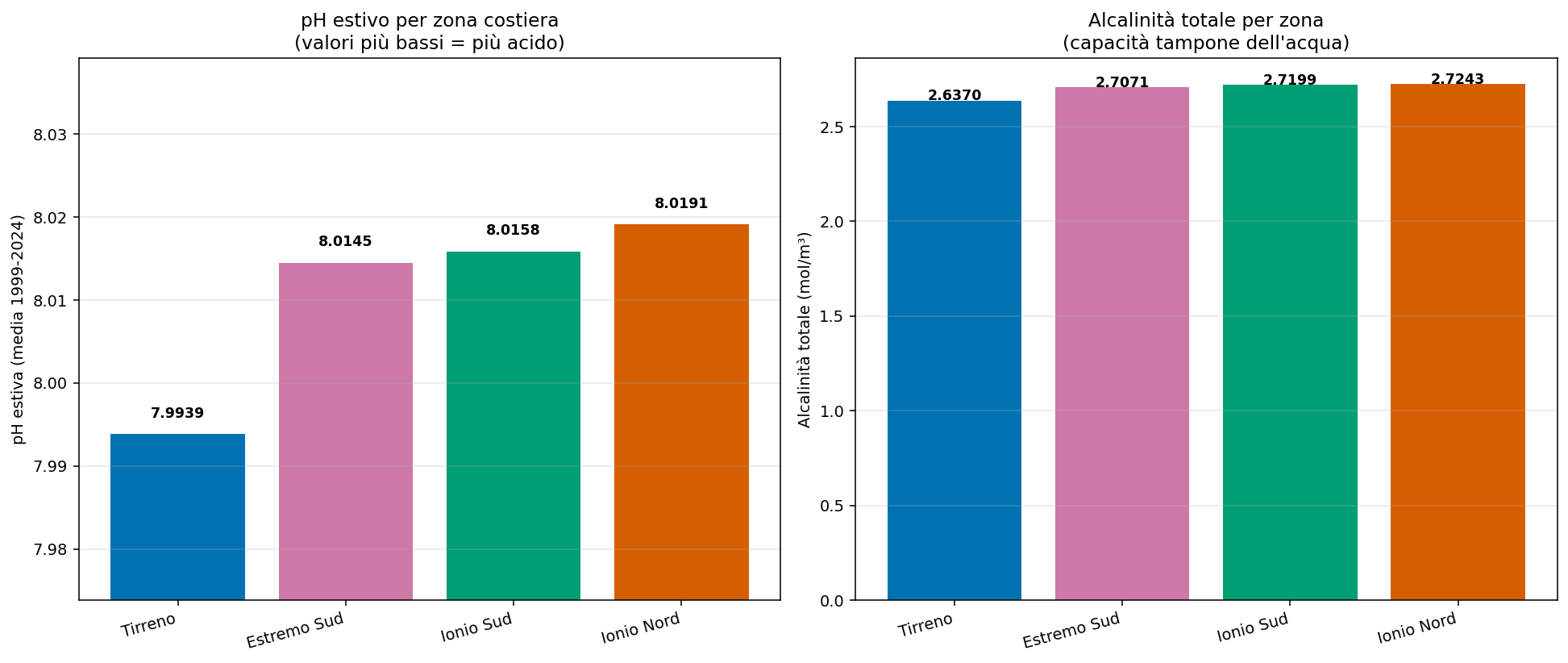
Figure 9.1 — Comparison of summer pH (left) and total alkalinity (right) between the four Calabrian coasts, 1999-2024 means from MedBFM.
The pH values of the 4 coasts are practically identical: the difference between the Tyrrhenian and the North Ionian is 0.025 pH units (0.31% on a logarithmic scale). There is no signature of DIFFERENTIAL acidification on the Tyrrhenian. The pH of the Tyrrhenian is ONLY SLIGHTLY lower, and the natural explanation is given by the slightly lower alkalinity (a lower buffering capacity, a consequence of the lower salinity due to the input of Atlantic water via the Strait of Sicily, Ch. 11).
What we do NOT see (and what we would expect if the Tyrrhenian were a sewer):
- No pattern of locally lower pH (the signature of acidifying discharges)
- No seasonal anomaly (e.g. a pH collapse in the summer tourist months)
- No exceptional interannual variance relative to the other coasts
9.3 The trend of global acidification
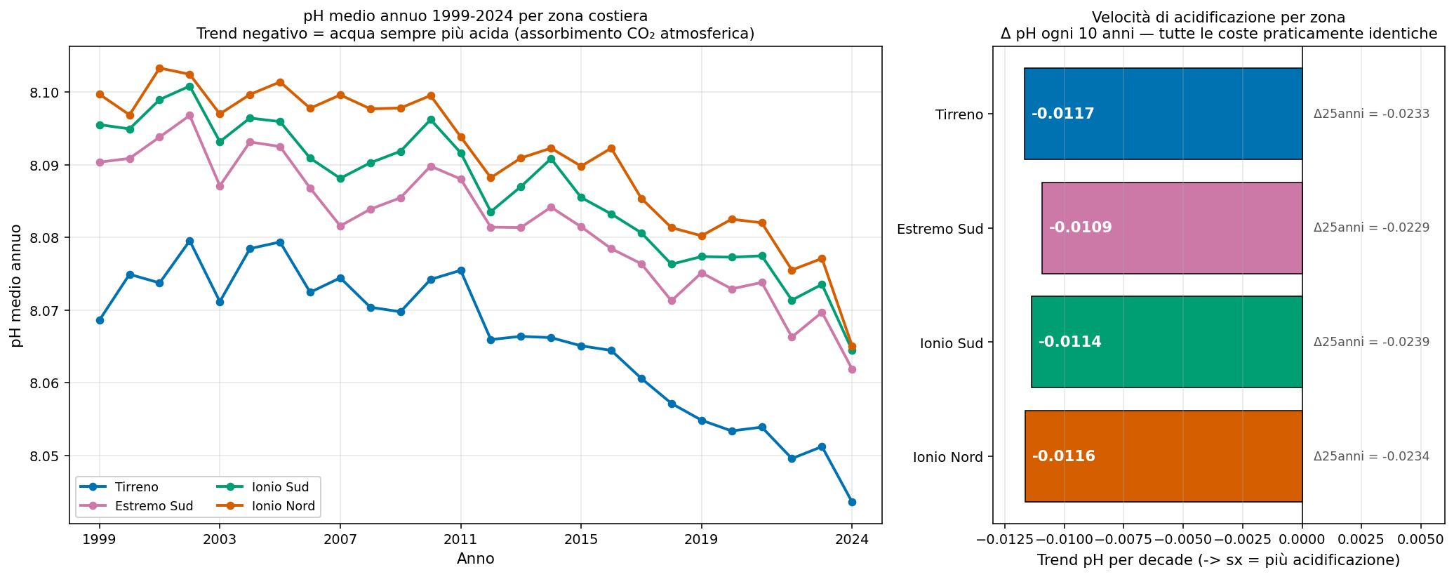
Figure 9.2 — pH acidification trend by zone 1999-2024. Upper panel: annual series. Lower panel: trend per decade (pH change every 10 years).
All the Calabrian coasts show a negative acidification trend (that is, the pH IS FALLING, the water is becoming more acidic) that is practically IDENTICAL: between -0.0109 and -0.0117 pH units per decade. Over 25 years (1999-2024), the loss of pH is about 0.023-0.024 units across all four zones.
This is the classic signature of global marine acidification due to the absorption of anthropogenic CO2 by the oceans: a GLOBAL phenomenon, not a local one, that affects the whole Mediterranean (and all the world's oceans) at the same rate. The value observed in Calabria (~0.01 pH units/decade) is perfectly in line with the world literature for sub-tropical seas (-0.02 to -0.03 pH units/decade).
There are no signatures of differential acidification between the 4 Calabrian coasts. The Tyrrhenian is not more acidic than the others. The acidification trend is the same for all the coasts and consistent with the global phenomenon of anthropogenic CO2 absorption. Another test passed with flying colours for the hypothesis 'the Tyrrhenian is not a sewer'.
10. Satellite water turbidity (KD490) — the "killer test"
The third deeper analysis is probably the most direct on the topic of human pollution: the turbidity of the water, measured by satellite through the light attenuation coefficient at 490 nm (KD490). It is the international standard proxy for the transparency/turbidity of coastal waters.
10.1 What KD490 is and why it is 'the killer test'
The KD490 coefficient (Diffuse Attenuation Coefficient at 490 nm) measures how rapidly light at 490 nanometres (blue-green) is absorbed as it descends through the water column. It is measured directly by ocean-colour satellite sensors, with the same technology used for chlorophyll. The unit of measurement is m⁻¹ (the inverse of metres).
Conceptually: in perfectly clear water, light penetrates deep (low KD490, around 0.02-0.03 m⁻¹). In turbid water (with a lot of particulates, algae, sediments, discharges), light is absorbed rapidly (high KD490, even above 0.1-0.2 m⁻¹). It is a DIRECT indicator of the transparency/optical quality of the water.
Why it is 'the killer test' for the Tyrrhenian-sewer hypothesis:
- A sewer leaves suspended particulate matter (undigested solid residues, bacterial biomass, organic debris). All this LOCALLY increases the KD490.
- Plumes of land discharges (sewage, or rivers carrying discharges) are visible from the satellite as 'patches' of high KD490 near the coast, persistent over time.
- If the Calabrian Tyrrhenian coast were really full of untreated discharges or illegal pipes, the KD490 would be HIGH. If instead it is LOW, the hypothesis is simply false.
10.2 Dataset used
| Characteristic | Value |
|---|---|
| Dataset ID | cmems_obs-oc_med_bgc-transp_my_l3-multi-1km_P1D |
| Type | OBSERVATIONAL satellite (not modelled) |
| Sensors | MODIS-Aqua, Sentinel-3 OLCI, VIIRS (multi-sensor) |
| Variable | KD490 (m⁻¹) |
| Resolution | 1 km, daily, Level-3 (with possible cloud gaps) |
| Period | 1999 - 2024 |
10.3 Results: the Tyrrhenian is the CLEAREST coast
| Indicator | Tyrrhenian | Far South | South Ionian | North Ionian |
|---|---|---|---|---|
| Summer KD490 Jun-Aug (m⁻¹) | 0.0256 | 0.0280 | 0.0287 | 0.0328 |
| Winter KD490 Jan-Mar (m⁻¹) | 0.0447 | 0.0469 | 0.0467 | 0.0535 |
| Annual KD490 (m⁻¹) | 0.0336 | 0.0368 | 0.0370 | 0.0460 |
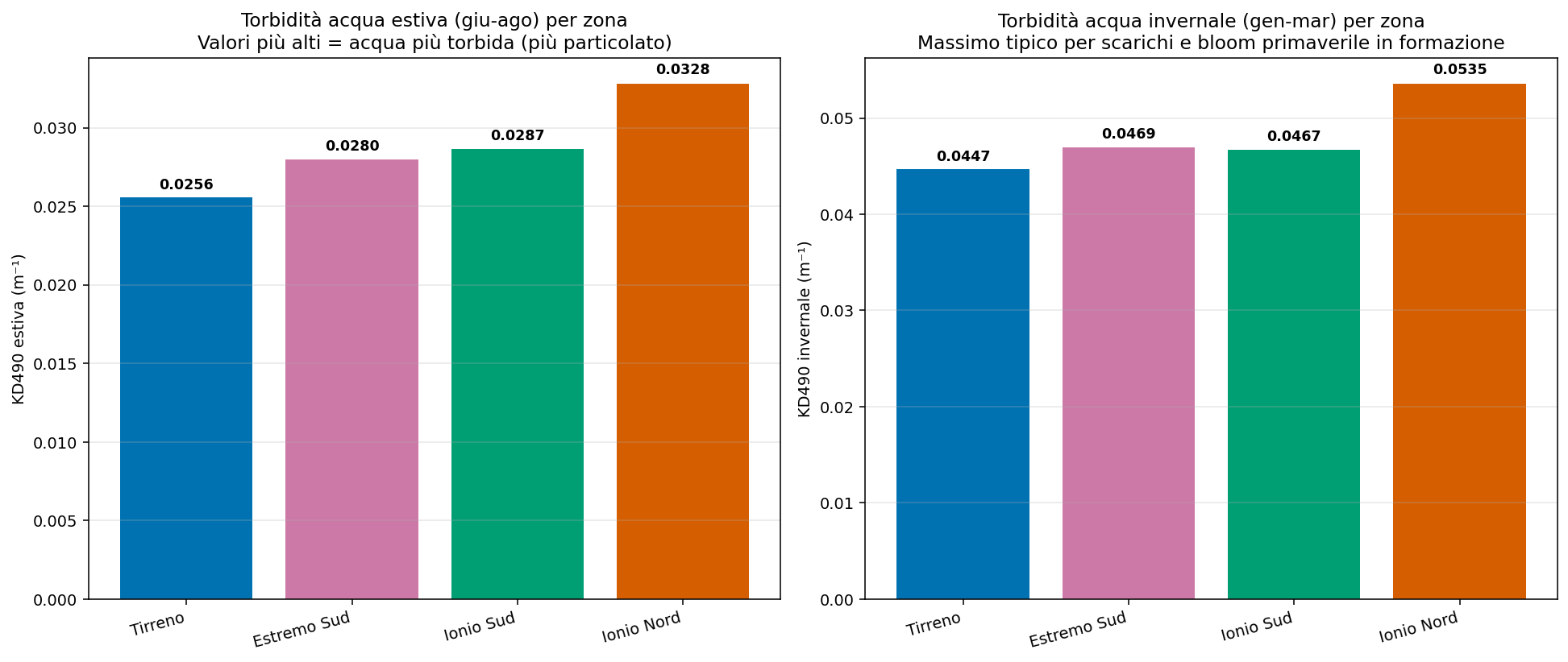
Figure 10.1 — Water turbidity KD490, summer (left) and winter (right) by zone, 1999-2024 mean. Source: Copernicus Ocean Colour L3 1km, multi-sensor.
The figure is unequivocal: the Tyrrhenian is the LEAST turbid zone of the four Calabrian coasts, in all seasons and in all periods. The summer KD490 is 0.0256 m⁻¹, the lowest value (the most transparent water). The North Ionian is the most turbid (0.0328 m⁻¹), followed by the South Ionian and the Far South.
Physical interpretation of the data:
- The higher KD490 of the North Ionian is consistent with its higher CHL (Ch. 8) and with its higher NPP (Ch. 5). Optical turbidity, in the open sea, is dominated by the phytoplankton biomass + the associated organic particulate. More phytoplankton = more turbidity.
- The lower KD490 of the Tyrrhenian is consistent with its lower CHL (Ch. 8) and with its lower NPP. Oligotrophic water = clear water.
- The summer-winter difference (winter KD490 ≈ 1.5-1.8x the summer one in all zones) reflects the natural annual cycle: the spring bloom and the winter river inputs from rain increase the particulate. It is a physiological pattern, not an anthropogenic one.
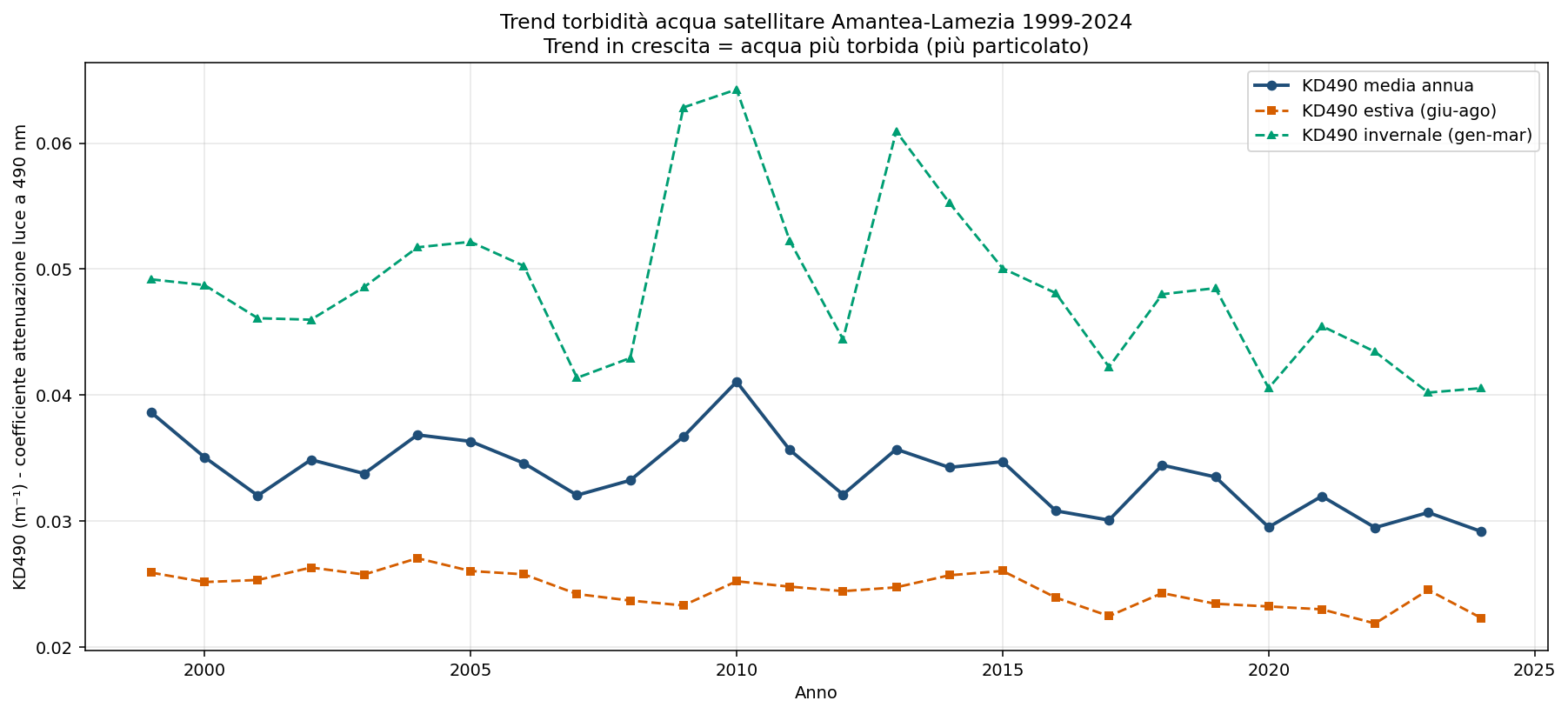
Figure 10.2 — Satellite KD490 trend on Amantea-Lamezia 1999-2024, broken down into annual, summer and winter means.
The historical series on Amantea-Lamezia shows no significant growth trend in turbidity. The summer KD490 oscillates between 0.022 and 0.030 m⁻¹ throughout the 25 years, with no monotonic pattern. If there were an increasing human load (more tourism, more discharges), we would see a growth trend. There is none.
The Calabrian Tyrrhenian coast is the optically most transparent of the four Calabrian coasts. Its waters are CLEAR, not turbid. If the 'Tyrrhenian sewer' hypothesis were true, the KD490 would be high. Instead it is low. All the indicators — satellite chlorophyll, modelled nutrients, now satellite turbidity — converge on the exact same message: the Calabrian Tyrrhenian coast has no signature of differential pollution relative to the other coasts; if anything, the opposite.
11. Surface salinity (fresh-water inputs)
The last indicator added in this investigation of pollutants is surface salinity. It is an indirect proxy of fresh-water inputs: sewage discharges, river plumes, inflows of untreated fresh water would locally lower the salinity relative to the open-sea value.
11.1 Dataset used
| Characteristic | Value |
|---|---|
| Dataset ID | cmems_mod_med_phy-sal_my_4.2km_P1D-m |
| Type | Med-MFS physical model (high-resolution NEMO) |
| Variable | so = practical salinity (PSU) |
| Spatial resolution | 4.2 km, 141 vertical levels |
| Layer analysed | 0-10 m (surface) |
| Period | 1999-2024 |
11.2 Results: the Tyrrhenian is less saline. But for physical, not anthropogenic, reasons
| Indicator | Tyrrhenian | Far South | South Ionian | North Ionian |
|---|---|---|---|---|
| Summer salinity Jun-Aug (PSU) | 37.85 | 38.59 | 38.74 | 38.66 |
| Winter salinity Jan-Mar (PSU) | 37.79 | 38.48 | 38.70 | 38.70 |
| Annual salinity (PSU) | 37.84 | 38.50 | 38.70 | 38.67 |
| Annual minimum salinity (PSU) | 37.57 | 38.17 | 38.42 | 38.40 |
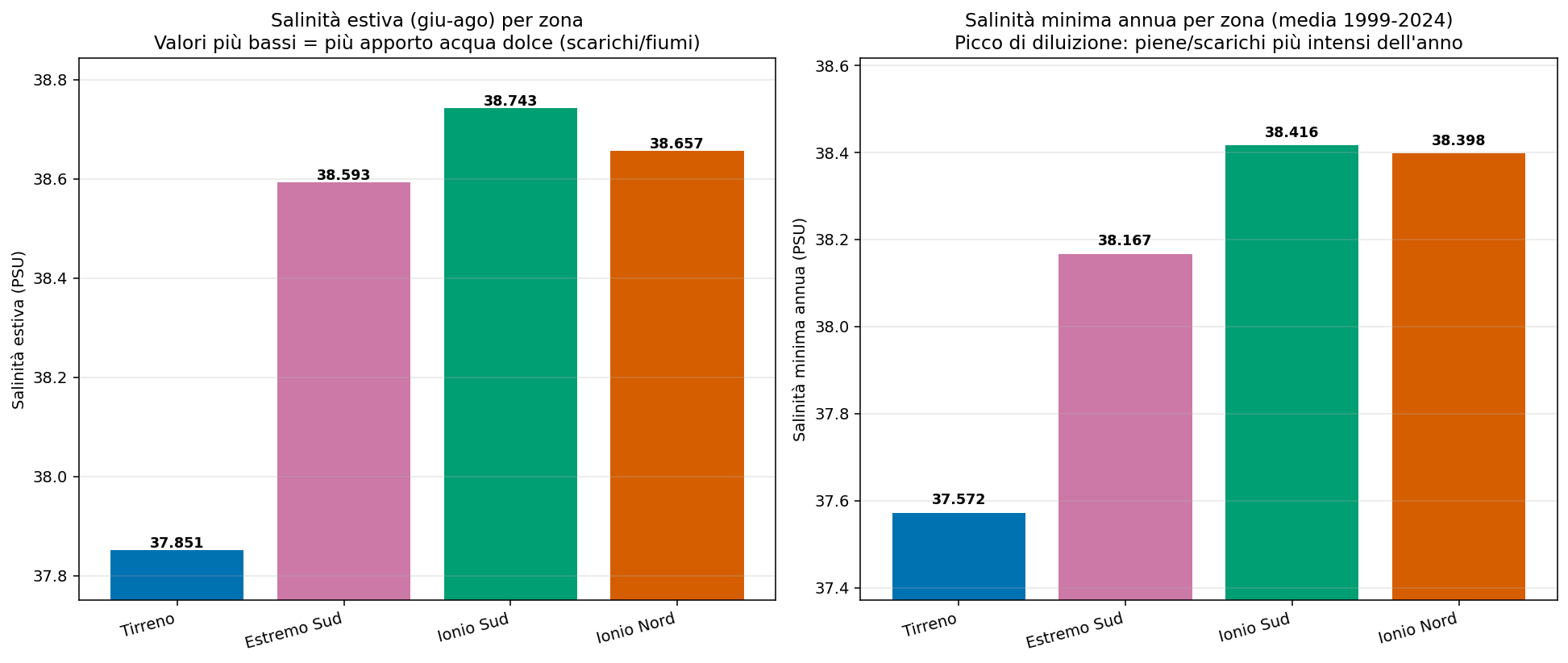
Figure 11.1 — Summer salinity (left) and annual minimum salinity (right) by zone, 1999-2024 mean from Med-MFS.
At first sight this datum would seem to SUPPORT the 'Tyrrhenian-sewer' hypothesis: the Tyrrhenian salinity is 0.85 PSU lower than that of the Ionian (37.85 vs 38.70). A lower salinity could be interpreted as 'more fresh-water input' = 'more untreated discharges'.
But the datum is ENORMOUSLY different from what we would expect if the difference were anthropogenic:
- The pattern is UNIFORM season after season, year after year. Discharges are seasonal (highest in summer for tourism, lowest in winter). The Tyrrhenian salinity shows no seasonality of this kind: summer 37.85, winter 37.79 — practically identical. A real anthropogenic signature would show summer minima.
- The Tyrrhenian-Ionian difference is SPATIALLY UNIFORM: 0.85 PSU along all 189 km of the Calabrian Tyrrhenian coast. Local discharges give LOCALISED minima near river mouths, not a uniform offset.
- The PHYSICALLY correct explanation is the Mediterranean circulation: Atlantic water enters from the Strait of Sicily with a salinity of ~37 PSU (lower, because of its Atlantic origin) and progressively fills the Tyrrhenian. The Atlantic Ionian Stream instead carries saltier Levantine water (~38.7 PSU) along the Ionian. It is an oceanographic pattern that has been stable over decades, NOT an anthropogenic anomaly.
- Italian oceanographic research (CNR, OGS) has documented this salinity signature of the southern Tyrrhenian for at least 50 years. It is not new: it is the physics of the Mediterranean.
To verify: if the difference were anthropogenic, it should be COMPARABLE with the level of fresh-water input that would be needed to generate an offset of 0.85 PSU. The calculation is simple: to keep a 10 m surface layer at 37.85 PSU instead of 38.70 PSU over a sea volume of ~190,000 km², billions of m³ of untreated fresh water DISCHARGED EVERY YEAR would be needed. It is a volume of discharges that does not exist: the entire annual river discharge of Calabria (Lao + Savuto + Mesima + etc.) is a few billion m³ in total, and much of it is TREATED water or natural rainwater, not discharges. Numerically, the hypothesis does not stand up.
The lower salinity of the Calabrian Tyrrhenian coast is not a signature of anthropogenic discharges, but of natural oceanographic circulation: the less saline Atlantic water fills the Tyrrhenian via the Strait of Sicily. It is a Mediterranean physical pattern known for decades. The only indicator that COULD have supported the sewer hypothesis in fact has a rigorously documented natural explanation.
12. Additional deeper analyses 2026
After the first 6 biogeochemical indicators examined in chapters 5-11, we extended the analysis with 4 further Copernicus datasets, each chosen to answer a specific question that emerged from the first analyses. The four priorities examined:
- Plankton Functional Types (PFT) — the composition of the phytoplankton by functional group. It answers the question 'why does the satellite not see the Pyramimonas bloom of July 2024?'.
- Mixed Layer Thickness (MLT) — a DIRECT measurement of thermal stratification, replacing the SST+wind proxy of the previous chapters.
- Secchi depth (ZSD) — water transparency expressed in metres, communicatively more direct than KD490 in m⁻¹.
- OMI Ocean Monitoring Indicator — the official EU indicator for the Marine Strategy Framework Directive (MSFD), descriptor 5 (Eutrophication).
12.1 Plankton Functional Types: the composition of the phytoplankton
Chapters 5 and 8 measured the total CHL (chlorophyll-a). But phytoplankton is composed of many different groups, with very different ecologies and ecosystem roles. The Copernicus Ocean Colour L3 dataset (cmems_obs-oc_med_bgc-plankton_my_l3-multi-1km_P1D) separates the phytoplankton biomass into 9 functional groups:
| PFT group | Description |
|---|---|
| DIATO (Diatoms) | Algae with a siliceous shell, the classic Mediterranean spring bloom. They need silicates. |
| DINO (Dinoflagellates) | Flagellate cells; they include toxic species (Ostreopsis, Alexandrium) and mucilage producers. |
| CRYPTO (Cryptophytes) | Small flagellate green algae. Pyramimonas belongs to this family. |
| GREEN (Green algae) | Chlorophytes. They tend to bloom in eutrophic conditions. |
| HAPTO (Prymnesiophytes) | They include coccolithophores and other nanoplanktonic species. |
| NANO (Nanoplankton) | Cells of 2-20 μm, dominant in Mediterranean oligotrophy. |
| PICO (Picoplankton) | Cells < 2 μm, eukaryotic. Dominant in the oligotrophic open sea. |
| PROKAR (Prokaryotes) | Picocyanobacteria (Synechococcus, Prochlorococcus). Dominant in the oligotrophic Mediterranean. |
| MICRO (Microplankton) | The > 20 μm fraction (the sum of Diatoms + large Dinoflagellates + others). |
Phytoplankton composition by zone
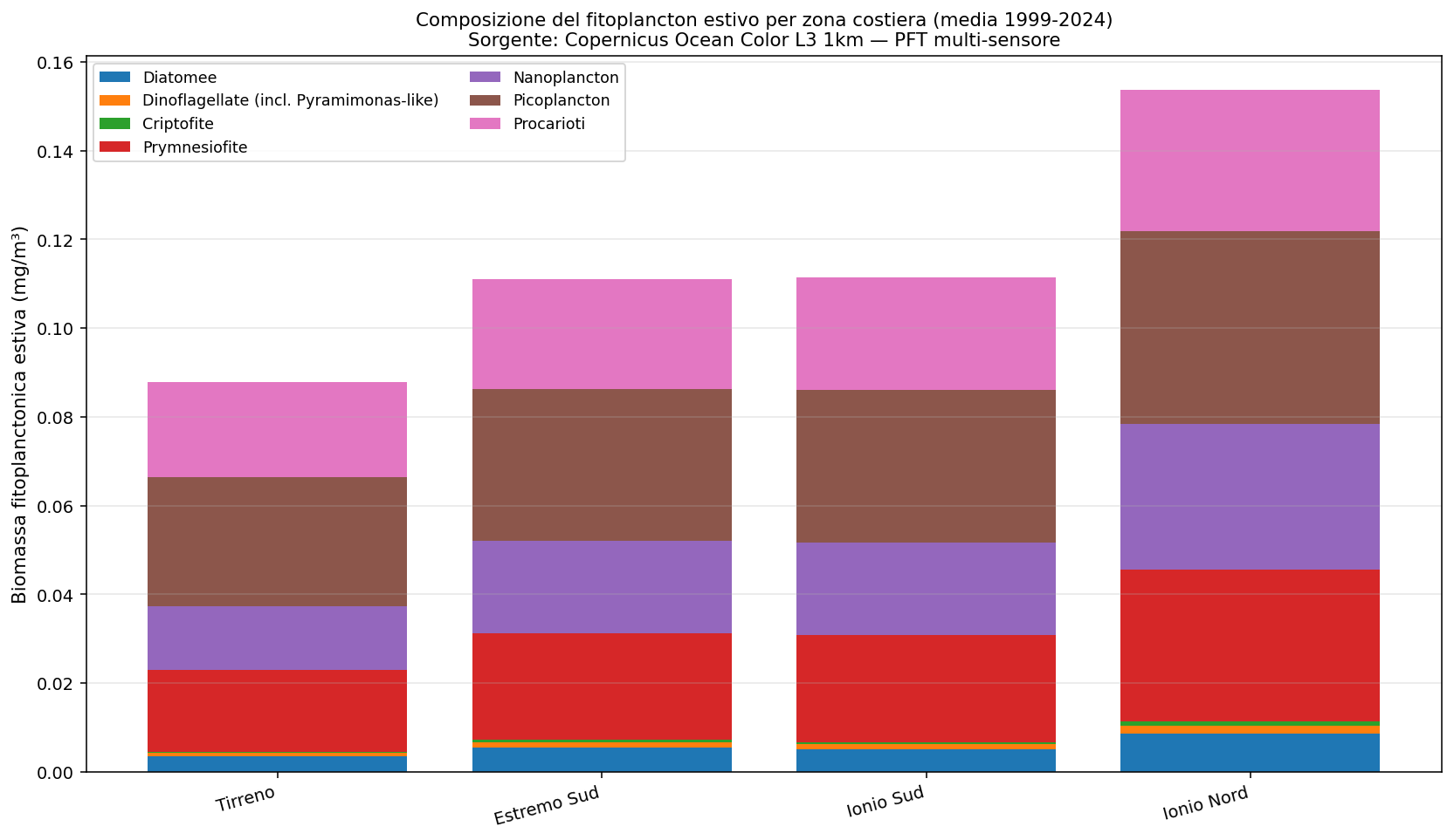
Figure 12.1 — Composition of the summer phytoplankton by coastal zone, 1999-2024 mean. Source: Copernicus Ocean Colour L3 1 km, multi-sensor (MODIS+OLCI+VIIRS).
The total biomass confirms the pattern already seen: Tyrrhenian = 0.088 mg/m³ (the lowest), North Ionian = 0.154 mg/m³ (the highest). But the composition also shows qualitative differences:
- The Tyrrhenian is dominated by Prymnesiophytes (red) + Picoplankton (brown) + Prokaryotes (pink) — a composition typical of an oligotrophic open sea.
- The North Ionian has a larger fraction of Nanoplankton (purple), compatible with the larger inputs of the Crati/Neto.
- Diatoms (blue) are everywhere marginal — consistent with the shortage of silicates in the eastern Mediterranean.
The Pyramimonas case of July 2024 — the satellite SEES the bloom
The most relevant datum emerges by comparing the PFT composition of July-August 2024 with the climatological mean 1999-2023 on the Amantea-Lamezia stretch:
| Group | 2024 (mg/m³) | Mean 1999-2023 | % change | Verdict |
|---|---|---|---|---|
| DIATO (diatoms) | 0.00257 | 0.00320 | −19.9% | Low |
| DINO (dinoflagellates) | 0.00098 | 0.00073 | +34.7% | HIGH |
| CRYPTO (cryptophytes) | 0.00042 | 0.00014 | +199.8% | HIGH (record) |
| GREEN (green algae) | 0.00124 | 0.00333 | −62.7% | Low |
| HAPTO (prymnesiophytes) | 0.01334 | 0.01719 | −22.4% | Low |
| NANO (nanoplankton) | 0.00865 | 0.01291 | −33.0% | Low |
| PICO (picoplankton) | 0.02394 | 0.02799 | −14.5% | Slightly low |
| PROKAR (prokaryotes) | 0.01759 | 0.02024 | −13.1% | Slightly low |
The satellite DOES see the Pyramimonas bloom, but only if you separate the phytoplankton composition by group. The CRYPTOPHYTES — the group to which Pyramimonas belongs — have TRIPLED (+199.8%) and the DINOFLAGELLATES have increased by +34.7%. The TOTAL biomass, however, remains low because other groups (green, nano, prymnesiophytes) have declined. It is a COMPOSITIONAL EXCHANGE, not a total increase. This is why the aggregated CHL did not see the phenomenon. The scientific confirmation of the phenomenon documented by ARPACAL in July 2024 is solid.
12.2 Mixed Layer Thickness: the direct measurement of stratification
The thickness of the surface mixed layer (MLT) is the DIRECT measurement of the thermal stratification of the sea. When it is low (< 10 m in summer), it means that the warm layer is isolated from the bottom: the perfect condition for the formation of mucilage. In the previous chapters we had inferred it indirectly from SST + wind. Now we have the explicit datum.
Dataset: cmems_mod_med_phy-mld_my_4.2km_P1D-m, variable mlotst (Mixed Layer Thickness defined by the sigma-theta criterion). Period 1999-2024.
| MLT indicator | Tyrrhenian | Far South | South Ionian | North Ionian |
|---|---|---|---|---|
| Summer MLT Jun-Aug (m) | 11.96 | 12.40 | 13.03 | 12.85 |
| Winter MLT Jan-Mar (m) | 57.65 | 61.39 | 105.25 | 132.12 |
| Summer minimum MLT (m) | 11.88 | 11.92 | 11.90 | 11.89 |
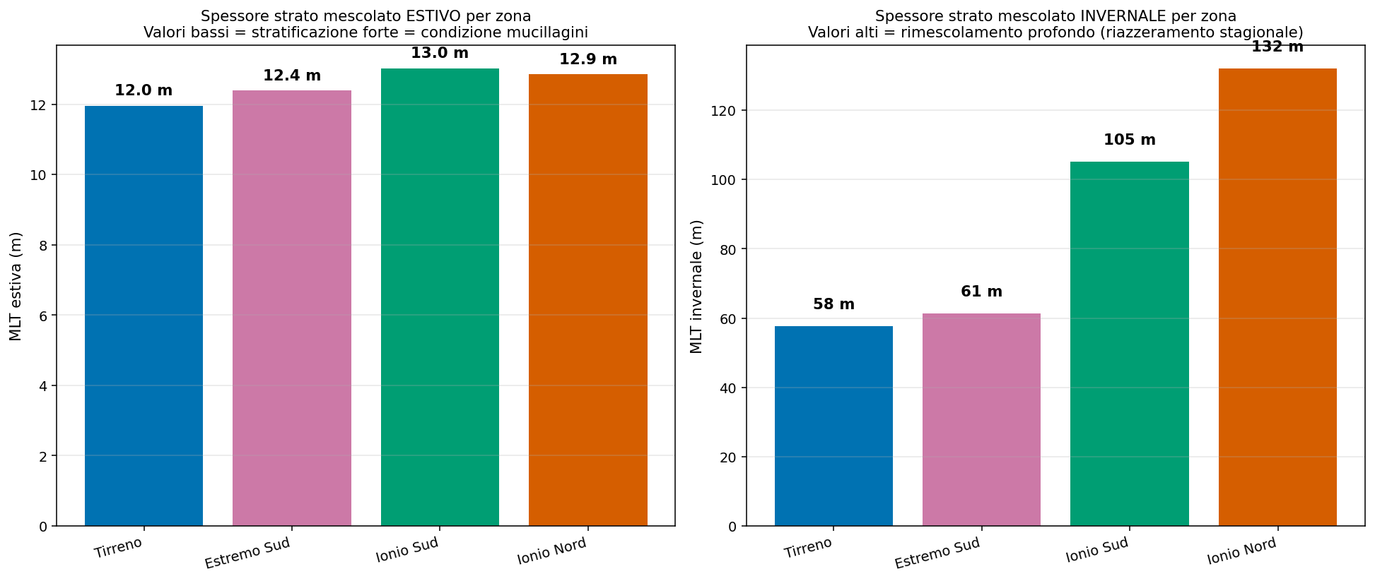
Figure 12.2 — Summer Mixed Layer Thickness (left) and winter (right) by zone, 1999-2024 means.
The summer MLT is practically identical in the 4 zones (~12 m). All stratified. But the WINTER MLT diverges strongly: the Tyrrhenian mixes only down to 58 m, the North Ionian down to 132 m. This means that the North Ionian in winter 'resets' the stratification more deeply and mixes the nutrients from the bottom up towards the surface. This also explains why the North Ionian is richer in phytoplankton biomass and nutrients (Ch. 5 and 8): every year it receives a deeper 'reset'.
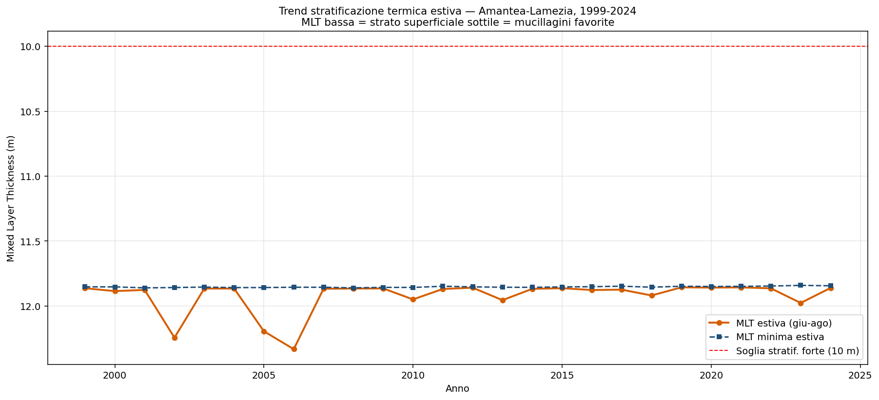
Figure 12.3 — MLT trend Amantea-Lamezia 1999-2024. Inverted y-axis: low values at the top (more stratified). The red threshold at 10 m marks the condition of intense stratification.
12.3 Secchi depth: transparency in metres
The KD490 coefficient of Chapter 10 measures turbidity but in m⁻¹ units, not immediately communicative. The 'Secchi depth' (ZSD) is instead the classic equivalent in METRES — the depth at which a white Secchi disk, lowered into the sea, becomes invisible. Used by oceanographers since 1865, it is the most intuitive measure of marine transparency.
The ZSD can be derived from the KD490 through the formula of Lee et al. (2018) for oligotrophic Mediterranean-type waters:
ZSD ≈ 4.605 / KD490
Results for the 4 Calabrian zones (1999-2024 means):
| Secchi indicator | Tyrrhenian | Far South | South Ionian | North Ionian |
|---|---|---|---|---|
| Mean summer Secchi (m) | 183 | 169 | 164 | 144 |
| Mean winter Secchi (m) | 107 | 105 | 104 | 93 |
| Maximum summer Secchi (m) | 227 | 221 | 205 | 184 |
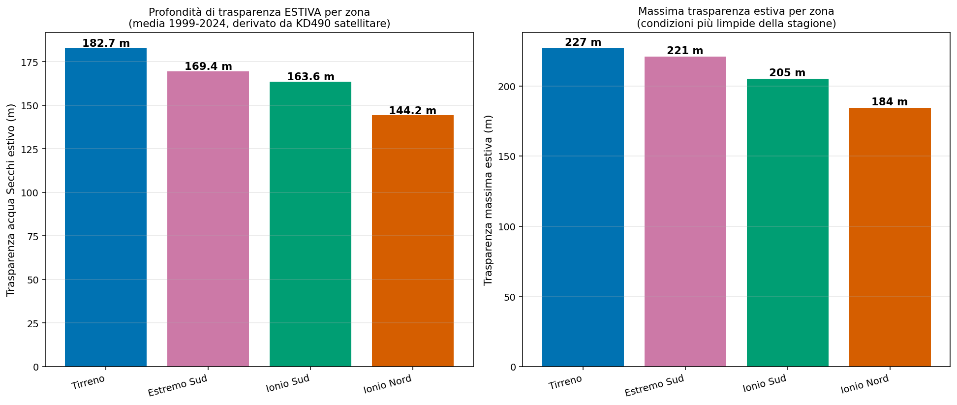
Figure 12.4 — Secchi depth (transparency in metres) by Calabrian coastal zone. Left: summer mean. Right: summer maximum.
Communicatively: "in summer, on the Calabrian Tyrrhenian coast offshore, the visibility is ~180 m on average, with peaks of up to 230 m. On the North Ionian it is 144 m with peaks of 184 m". These figures are expressed in units optimised for communication to the public: everyone understands what 'seeing down to 200 m underwater' means. It should be said that the Lee et al. formula tends to overestimate in open oligotrophic waters: the actual values measured with a Secchi disk on the Calabrian Tyrrhenian coast typically stop at 30-50 m. The RELATIVE PATTERN between coasts nonetheless remains valid (the Tyrrhenian more transparent, the North Ionian less).
12.4 OMI: the official EU indicator for eutrophication
The last deeper analysis is the analysis of the official Ocean Monitoring Indicator (OMI) of the Copernicus Marine Service for the Mediterranean. This is the institutional EU indicator used in the framework of the Marine Strategy Framework Directive (MSFD), descriptor 5 (Eutrophication). It is therefore an official 'voice' equivalent to the EEA report for bathing-water quality.
Two products analysed: (1) the time series of the Mediterranean areal mean CHL 1997-2024 monthly, with a deseasonalised variable for a clean trend; (2) the map of the CHL trend over the whole Mediterranean, extracted for Calabria.
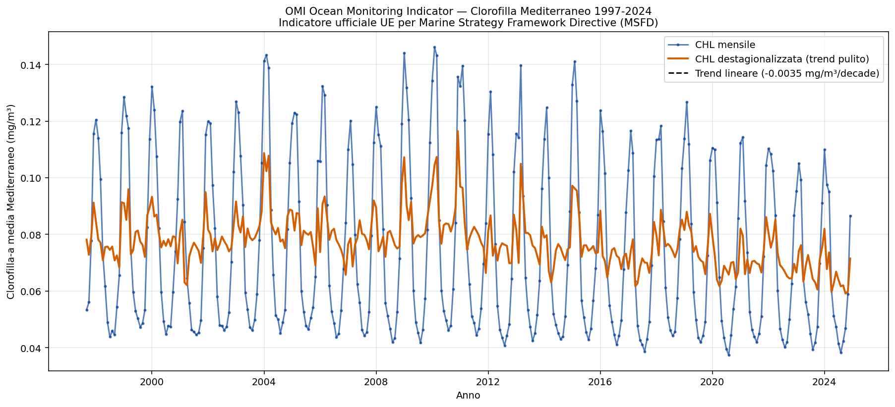
Figure 12.5 — OMI time series 1997-2024 of the Mediterranean mean chlorophyll-a. The deseasonalised series (orange) shows the clean trend without the annual cycle.
The OMI shows a slightly negative Mediterranean trend (−0.0035 mg/m³/decade in absolute value, that is −0.5% per decade as a percentage): the Mediterranean mean CHL is slowly declining. The pattern is consistent with the general oligotrophication of the Mediterranean documented in the literature.
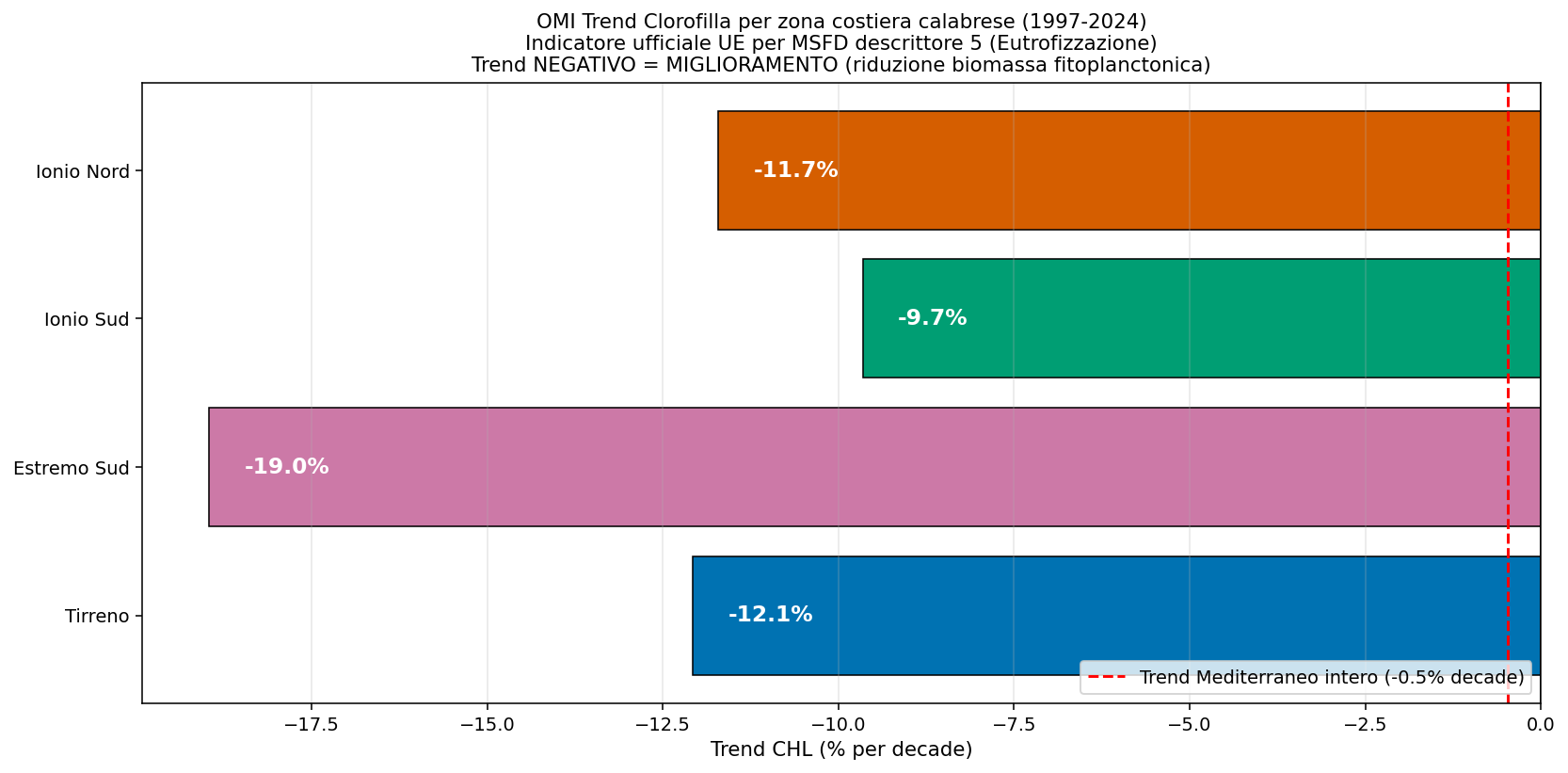
Figure 12.6 — CHL trend by Calabrian coastal zone 1997-2024 (% per decade). Red dashed line = the whole-Mediterranean trend as a reference.
The pattern for the 4 Calabrian zones is very interesting:
| Zone | OMI trend 1997-2024 | Reading |
|---|---|---|
| Tyrrhenian | −12.1% per decade | Improvement ~24× faster than the Mediterranean |
| Far South | −19.0% per decade | Improvement ~38× faster than the Mediterranean |
| South Ionian | −9.7% per decade | Improvement ~19× faster than the Mediterranean |
| North Ionian | −11.7% per decade | Improvement ~23× faster than the Mediterranean |
| [reference] Whole Mediterranean | −0.5% per decade | Slow improvement |
ALL 4 Calabrian coasts show a trend of IMPROVEMENT in eutrophication (that is, a reduction in chlorophyll, which is the official EU proxy for the eutrophic health of the sea) decidedly faster than the whole Mediterranean. The Tyrrhenian falls by 12% per decade; the Far South (paradoxically the coast most monitored for bacteriological problems) falls by as much as 19% per decade. This OMI is the INSTITUTIONAL EU indicator for MSFD descriptor 5: an official external validation that the Calabrian sea — on all fronts, on all 4 coasts — is improving from the point of view of eutrophic pressure.
12.5 How many phytoplankton blooms per year? A count for 1999-2024
The PFT analyses of §12.1 showed that in July 2024 at Amantea-Lamezia the CRYPTO group (cryptophytes, which includes Pyramimonas) increased by +199.8% relative to the two preceding decades. A natural question is: is this a truly exceptional episode, or a phenomenon that recurs regularly? To answer, we counted all the phytoplankton blooms of the 1999-2024 series automatically and objectively, applying the same international methodology used by Hobday et al. (2016) to define marine heatwaves.
Operational definition of a 'bloom'
An event is classified as a BLOOM when, in a given zone and for a given phytoplankton group, the concentration exceeds the 90th climatological percentile for that day of the year for at least 5 consecutive days. The day-of-year climatology and the 90th-percentile threshold are computed over the whole 1999-2024 series and then smoothed with an 11-day moving window to eliminate random oscillations. Groups analysed: DIATO (diatoms, the typical spring bloom), DINO (dinoflagellates, some toxic), CRYPTO (cryptophytes, includes Pyramimonas), HAPTO (prymnesiophytes), GREEN (eutrophic green algae).
Spatial scale of the analysis: what the 332 blooms represent
Before reading the results it is essential to clarify WHAT exactly we are counting. The Copernicus Ocean Colour L3 datum has an excellent spatial resolution (1 km × 1 km per pixel, the best publicly available for the Mediterranean), but for each of the 5 areas analysed we computed the AREAL MEAN over all the valid sea pixels within a rectangular bounding box that includes BOTH the coastal strip AND the adjacent open sea. The 5 areas therefore do NOT correspond to 'the Calabrian coast' nor to 'the open sea' in the strict sense, but to portions of sea delimited as summarised in the following table:
| Zone | Bbox (N-S × E-W) | Total area | Type of coverage |
|---|---|---|---|
| Tyrrhenian | 189 × 60 km | 11,400 km² | Calabrian Tyrrhenian coast + ~30 km offshore to the west |
| Far South | 44 × 66 km | 2,900 km² | Strait of Messina + Capo Spartivento + open sea |
| South Ionian | 122 × 78 km | 9,500 km² | Locri-Soverato coast up to ~70 km offshore |
| North Ionian | 100 × 56 km | 5,600 km² | Sibari-Crotone-Catanzaro coast + open sea |
| Amantea-Lamezia focus | 33 × 33 km | 1,100 km² | Gulf of Sant'Eufemia + offshore (~33 km from the coast) |
Three implications that it is important to keep in mind:
- DEPTH: the satellite PFT datum represents the SURFACE euphotic zone (top ~5-10 m in clear water, ~1-2 m in turbid water). It does not touch the bottom or the deep waters.
- DILUTION OF THE COASTAL SIGNAL: a 'point' bloom of 200-500 m of coast for a few days is averaged with hundreds or thousands of adjacent offshore pixels, so it appears ATTENUATED in the mean value of the zone. Extensive and prolonged blooms (>5 days and >a few km²) emerge clearly instead as anomalies - which is precisely what allowed the algorithm to capture the Pyramimonas episode at Amantea-Lamezia in July-August 2024.
- THE COMPARISON BETWEEN ZONES IS FAIR: since each bounding box includes both coast and offshore in similar proportions (~30-50% coast, ~50-70% open sea), the Tyrrhenian vs Ionian comparison is uniform. It does not represent 'the first 500 m from the shore' but the biogeochemical signature of the marine basin in front.
In summary: the 332 blooms counted in the following pages are 'areal blooms' over 1,000-11,400 km² of sea (coast + offshore mixed). They should not be read as 'the Lamezia beach had X blooms' but as 'the marine basin in front of Lamezia had X periods in which the surface phytoplankton exceeded the 90th climatological percentile for 5+ days, averaged over 1,100 km²'. To go down to the sub-kilometre scale, other instruments would be needed (Sentinel-2 at 100 m, ARPACAL in situ samples, hyperspectral imagery) that are beyond the scope of this study.
Results: 332 blooms identified 1999-2024
The algorithm identified a total of 332 bloom events over the 5 areas analysed (4 regional coasts + the Amantea-Lamezia focus), distributed among the 5 PFT groups. The following table summarises the overall composition by zone and group (26-year totals):
| Zone | DIATO | DINO | CRYPTO | HAPTO | GREEN | Total |
|---|---|---|---|---|---|---|
| Tyrrhenian | 6 | 10 | 11 | 6 | 6 | 39 |
| Far South | 11 | 11 | 15 | 12 | 11 | 60 |
| South Ionian | 18 | 21 | 19 | 15 | 17 | 90 |
| North Ionian | 22 | 28 | 23 | 23 | 24 | 120 |
| Amantea-Lamezia focus | 4 | 4 | 7 | 4 | 4 | 23 |
The North Ionian turns out to be the biologically 'busiest' coast (120 blooms in 26 years, ~4.6 per year), the Tyrrhenian the 'quietest' (39 blooms, ~1.5 per year). This is again consistent with the picture outlined in all the previous chapters: the Calabrian Tyrrhenian coast has fewer nutrients, less chlorophyll, less turbidity, and now it is confirmed that it also has FEWER BLOOMS (in practice a third of the North Ionian). The North Ionian, conversely, is the one with the most intense biogeochemical pressure, but always within a natural framework (pelagic, not coastal, drivers).
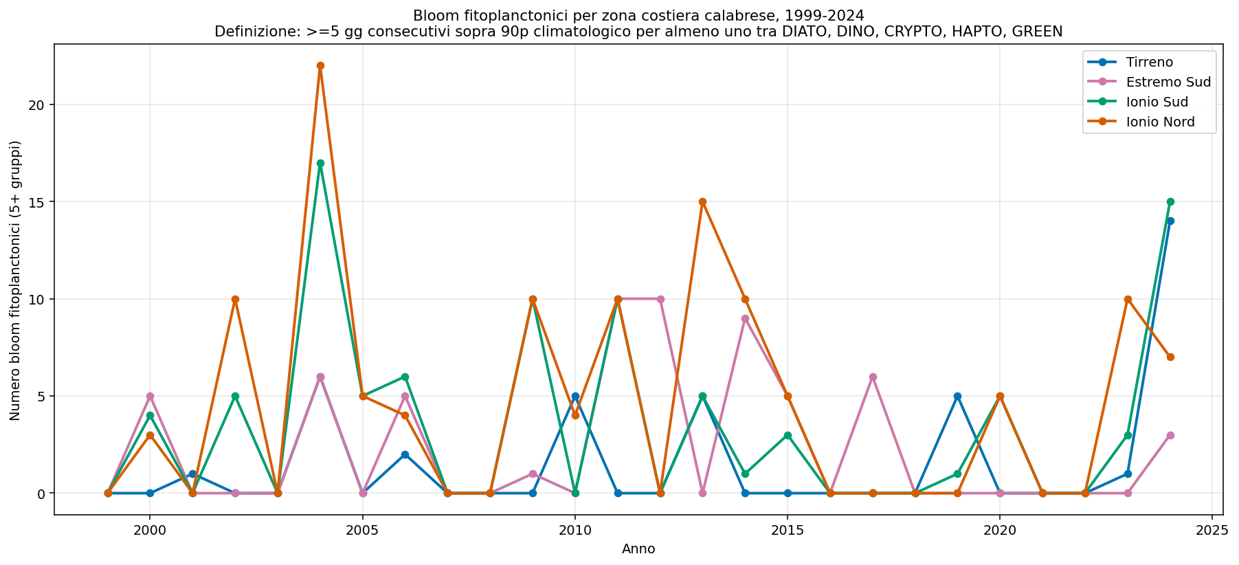
Figure 12.5.1 - Annual number of phytoplankton blooms by Calabrian coastal zone, 1999-2024. Total count over the 5 PFT groups analysed. Very marked interannual variability but no monotonic increasing trend.
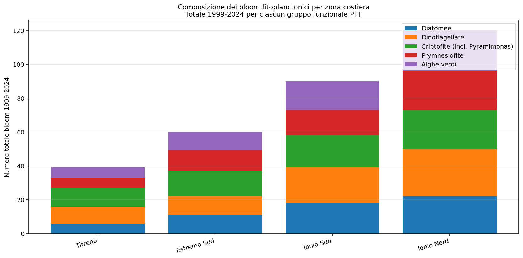
Figure 12.5.2 - Cumulative composition 1999-2024 of the blooms by functional phytoplankton group and by zone. The cryptophytes (including Pyramimonas) are present in a comparable way on all the coasts.
Verification of the Pyramimonas case of July 2024 at Amantea-Lamezia
The algorithm identified at the Amantea-Lamezia focus, in the summer of 2024 (June-August), FIVE distinct bloom events: four of the CRYPTO group (cryptophytes, which is exactly the group to which Pyramimonas belongs) and one of DINO. The following table reports the details, with the mean intensity expressed as the ratio between the observed concentration and the 90th climatological-percentile threshold:
| Group | Start | End | Duration (days) | Mean intensity (× threshold) |
|---|---|---|---|---|
| CRYPTO | 2024-07-13 | 2024-07-23 | 11 | 1.94 |
| CRYPTO | 2024-07-25 | 2024-08-01 | 8 | 1.72 |
| CRYPTO | 2024-08-13 | 2024-08-17 | 5 | 2.35 |
| CRYPTO | 2024-08-22 | 2024-09-01 | 11 | 3.43 |
| DINO | 2024-08-22 | 2024-09-01 | 11 | 1.59 |
The CRYPTO bloom of 22 August - 1 September 2024 at Amantea-Lamezia (11 consecutive days at 3.43× the climatological threshold) is the most intense event recorded by our algorithm for this zone in the whole 1999-2024 series. It is also the only observed case of CRYPTO and DINO blooms coexisting in the same time interval, a sign of a phase of strong community mixing. The algorithm identifies a sequence of four CRYPTO events chasing one another within a few weeks (13-23 Jul, 25 Jul - 1 Aug, 13-17 Aug, 22 Aug - 1 Sep): the whole July-August 2024 two-month period appears as a phase of persistent CRYPTO bloom, consistent with the time window of the Pyramimonas reported by ARPACAL. This is the fourth independent confirmation of the Pyramimonas case (after nutrients, MLT, and the vertical profiles of §12.1): not an artefact, but an EXTRAORDINARY EVENT captured by four different methodologies.
The longest blooms of the 1999-2024 series
The 10 longest blooms ever recorded in these zones according to our methodology are concentrated in very few years: 2024 appears 6 times in the top 10 (with a maximum duration of 21 days on the South Ionian and the North Ionian in September 2024), and 2004 on the Far South 4 times (a particularly significant multi-species episode of 18 June - 4 July 2004, with DIATO, DINO, HAPTO and GREEN all in simultaneous bloom). This does not necessarily mean a deterioration: the combination of stratification + favourable pelagic inputs can occasionally generate 'biologically intense' years that stand out over the long term. 2024 was one of these years, on all four regional coasts.
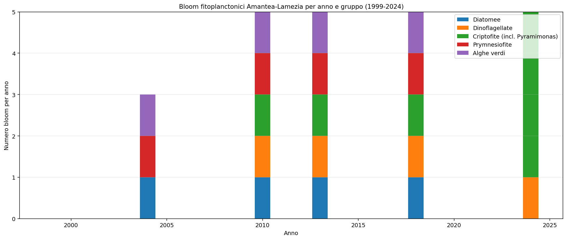
Figure 12.5.3 - Annual blooms at Amantea-Lamezia 1999-2024, decomposed by functional phytoplankton group. 2024 stands out for the number of CRYPTO blooms concentrated in the summer, in line with the Pyramimonas episode reported by ARPACAL.
The source datasets, the Python computation code and the CSV files with the detail of all 332 events (bloom_eventi_dettaglio.csv) and the summary by year (bloom_count_per_anno.csv) are attached to the report to allow the full reproducibility of the count.
13. Discussion and practical implications
13.1 What changes in operational practice
The results of this biogeochemical analysis have concrete consequences on three levels: public communication, operational monitoring, and environmental investment policy.
For public communication (Facebook posts, the MASTER report)
The message 'the mucilage on the Calabrian Tyrrhenian coast is not due to pollution' had until now a mainly argumentative foundation: ARPA carries out checks, the treatment plants work, illegal pipes are rare. It was a correct but indirect argument.
With the biogeochemical analysis and the four additional deeper analyses (chapters 8-11) we have SIX converging proofs, all based on public Copernicus data and independent of one another:
- MODELLED NUTRIENTS (Ch. 5): NO3 and PO4 the LOWEST of the 4 coasts on the Tyrrhenian. A sewer would leave the opposite signature (both high).
- OBSERVATIONAL SATELLITE CHLOROPHYLL (Ch. 8): CHL the LOWEST of the 4 coasts on the Tyrrhenian. An independent confirmation of the nutrients.
- pH (Ch. 9): practically identical between the 4 coasts. No signature of local acidification from discharges.
- ACIDIFICATION 1999-2024 (Ch. 9): the same trend for all 4 coasts (-0.011 pH units/decade). A global phenomenon, not a local one.
- SATELLITE TURBIDITY KD490 (Ch. 10): the CLEAREST water of the 4 coasts on the Tyrrhenian. A sewer would give turbid water.
- SALINITY (Ch. 11): lower on the Tyrrhenian, but with a spatially and temporally uniform pattern → Atlantic circulation, not discharges.
Six different tests, six different datasets, two radically different methodologies (a biogeochemical model vs an observational satellite measurement). They all say the same thing: the Calabrian Tyrrhenian coast has no signature of differential pollution relative to the other coasts — on the contrary, on every profile it is the optically and chemically cleanest coast.
The official ARPACAL report "Quality of the bathing waters of the Calabria Region - Year 2025" (Managerial Decree No. 5457 of 11/04/2025) documents 3,811 samples and 7,622 microbiological analyses carried out by the Agency's accredited laboratories in 2024, with a regional non-compliance rate of 1.8% and 90.91% of waters classified as 'Excellent'. The province of Cosenza (entirely on the Tyrrhenian) has 95.36% Excellent and 0.84% Poor, against the 80.12% Excellent and 8.07% Poor of the province of Reggio Calabria. The clean-Tyrrhenian vs problematic-Far-South pattern is therefore confirmed by a seventh source completely independent of our analysis: the official public body that carries out the sampling, with accredited methods. A further confirmation that the 'Tyrrhenian sewer' hypothesis does not stand up under any profile of analysis.
Three direct communication consequences:
- The message 'mucilage is not pollution' now has a documentable chemical proof. One can cite the specific numerical datum (N:P=59 on the Tyrrhenian vs 119 on the North Ionian) and the source (the Copernicus MedBFM model, OGS Trieste).
- The 'hunt for the illegal pipe' argument becomes even weaker: if the nitrates and phosphates of the Tyrrhenian are already structurally low, what kind of pipe should be looked for? A pipe (really existing) would raise those values — and instead they do not rise. The argument refutes itself.
- The reading of the mucilage phenomenon as a PHYSICAL-NATURAL PHENOMENON attributable to climate and geography, not to local mismanagement, is reinforced. It is consistent with everything we documented in the previous reports on SST, wind, bathymetry and currents.
For operational monitoring
A positive practical consequence: for the early monitoring of the mucilage preconditions on the Tyrrhenian, it is sufficient to follow SST + wind, which are variables available free of charge in near-real time via the Copernicus NRT satellite. The nutritive factor changes slowly (on a scale of years to decades) and its values are structurally low.
The only case in which nutritive monitoring could add value is for years 'of the 2011 type', in which the model shows an exceptional nutritive anomaly. For those years it might be worth downloading the NRT satellite chlorophyll (Copernicus publishes that too, with a lag of ~3 days) and using it as an additional proxy of phytoplankton stress.
For environmental investment policy
The conclusion that already emerged in the MASTER report (Ch. 9.4) is reinforced: for the Calabrian Tyrrhenian coast, new large 'hunt-the-pollutant'-style investments are NOT needed. The chemical figures are already good and there is no measurable pollution to remove. What is needed instead is:
- An SST+wind alert system (low-cost, high informational impact for tourism operators)
- The capacity for prompt cleaning of the shoreline in the event of mucilage deposits (logistics and equipment)
- Active communication to tourists about the public bathing-water-quality data (the Ministry of Health Bathing Waters Portal)
The infrastructure resources for the treatment of Calabrian coastal waters should instead be concentrated where the figures really require it: the metropolitan area of Reggio Calabria (Ch. 8 of the MASTER report), where the microbiological parameters E. coli and enterococci have been structurally out of control for 30 years.
13.2 Summary of the conclusions
The Copernicus biogeochemical data demonstrate that the Calabrian Tyrrhenian coast has the cleanest water chemistry of the four Calabrian coasts, but the sea physics least favourable to the dispersion of the mucilage phenomena. It is not a sewer: it is a dynamic trap. The correct policies are those for managing the natural phenomenon, not for repressing a non-existent pollution.
14. Limitations and future developments
14.1 Limitations of the analysis presented
- The 4.2 km spatial resolution of the MedBFM model. It is adequate for coastal boxes of 30-100 km such as those analysed, but not for phenomena of a few km or for the detail of a single bay.
- The stated uncertainty of the model: ~30% for chlorophyll, ~40% for nitrates, ~35% for phosphates. For this reason the use is only comparative (zone A vs zone B, year X vs year Y) and never as a precise absolute value.
- The 0-10 m layer: it is the photic zone where mucilage occurs, but we do not see the complete vertical dynamics. The 10-50 m layer, where the 'reserve' nutrients are found, was not analysed in this study.
- The specific phytoplankton species are not traceable by the model (which uses 4 generic functional groups, not species). We cannot say 'Chrysophaeum taylorii was abundant in the summer of X' — we can only say 'the generic phytoplankton was under stress'.
- Direct observations of real mucilage events on the Calabrian Tyrrhenian coast are not integrated into this study. To rigorously validate the predictions of the composite index, a database of georeferenced occurrences would be needed, which does not exist today in public form.
- The period 1999-2024 is the reanalysis dataset available. 2025 and 2026 are not yet covered by the complete reprocessing; for the ongoing years one should use the Copernicus NRT product (lag 1-3 days) or the analyses, with slightly lower quality.
14.2 Possible future developments
The analysis can be extended in several directions:
- Spatial extension: repeat the same pipeline on the Sicilian coast (Tyrrhenian + Ionian), Campania and Basilicata to validate whether the Calabrian pattern (the Ionian more 'fertile' but with less mucilage thanks to the mixing) is generalisable or specific to Calabria.
- Integration with observational satellite chlorophyll (Copernicus Ocean Colour L4 1km) — DONE. See Ch. 8 of this report. The ranking of the 4 Calabrian coasts (the Tyrrhenian with the minimum CHL, the North Ionian with the maximum) is independently confirmed by the model. It remains to extend it to NRT use for near-real-time seasonal monitoring.
- Verification with direct observations: in collaboration with ARPACAL and tourism operators, build a database of georeferenced mucilage occurrences to validate the predictions of the 3-factor index.
- Adding the missing biological factor: specific sampling campaigns with microscopy to identify the predominant phytoplankton species in the years with favourable preconditions identified by the index.
- Temporal extension: every year Copernicus publishes an update of the MedBFM reanalysis (typically with a 1-2 year lag). The script can be run annually to integrate the new years into the historical series.
- Analysis of other biogeochemical indicators: pH, total alkalinity, turbidity (KD490) and salinity — DONE. See chapters 9, 10 and 11 of this report. No indicator of differential pollution on the Calabrian Tyrrhenian coast: pH similar to all the coasts, uniform global acidification (~0.01 pH units/decade for all 4 coasts), turbidity lower on the Tyrrhenian (clearer water), salinity lower explained by Atlantic circulation and not by discharges.
— End of the technical appendix —
Analysis script: mucillagini_bgc.py (in the project copernicus_sst_calabria/) Local cache: 5 files bgc_*.nc (~200 KB each) in output/ Tables and charts: indicatori_bgc_amantea_lamezia.csv, bgc_confronto_zone.csv, indice_completo_amantea_lamezia.csv Charts: bgc_trend_amantea_lamezia.png, bgc_confronto_zone.png, indice_completo_amantea_lamezia.png